2.1 本章學習目標
讀完本章後,你應該能夠:
- 說明連續型結局 (continuous outcome) 中平均差 (mean difference, MD) 與標準化平均差 (standardised mean difference, SMD) 的使用情境。
- 寫出固定效應模型 (fixed-effect model) 的加權平均概念。
- 解釋隨機效應模型 (random-effects model) 如何納入研究間變異 (between-study variance)。
- 計算並解讀 \(\tau^2\)、\(I^2\)、\(Q\) 檢定、Hartung–Knapp 調整與預測區間 (prediction interval)。
- 執行一個簡單的次族群分析 (subgroup analysis),並知道它可以幫忙思考異質性,但不能隨便變成「故事生成器」。
上一章我們用二元結局示範統合分析的基本精神。本章開始進入標準方法的主菜:如果每篇研究的結果不完全一樣,我們到底要把它們視為「同一個真實效果的不同抽樣誤差」,還是「不同研究可能真的有不同效果」?
這個問題就是固定效應與隨機效應模型的核心。它看起來像統計技術選擇,其實也很像臨床判斷:同樣是降血壓介入,醫學中心、社區診所、偏鄉衛教、數位照護,真的會完全一樣嗎?如果你心裡浮出「嗯,很難吧」,恭喜,你已經站在隨機效應模型的門口。
2.2 連續型結局的效果量
連續型結局 (continuous outcome) 是以數值尺度測量的結局,例如收縮壓、低密度脂蛋白膽固醇、疼痛量表分數、憂鬱量表分數、住院天數等。
2.2.1 平均差
平均差 (mean difference, MD) 適合用在所有研究使用相同單位與相同量表時。例如所有研究都回報 12 週後收縮壓相對基準值的變化,單位都是 mmHg,這時候 MD 很直覺:
\[
MD_i = \bar{X}_{T,i} - \bar{X}_{C,i}
\]
其中 \(\bar{X}_{T,i}\) 是第 \(i\) 個研究介入組平均值,\(\bar{X}_{C,i}\) 是對照組平均值。本章範例中,結局是 12 週收縮壓變化;數值越負,代表血壓下降越多,所以 MD < 0 代表介入組比對照組降更多。
Code
ci_norm <- function(theta, se, level = 0.95) {
  z <- qnorm(1 - (1 - level) / 2)
  c(lower = theta - z * se, upper = theta + z * se)
}

meta_iv <- function(yi, sei) {
  vi <- sei^2
  k <- length(yi)
  w_fe <- 1 / vi
  theta_fe <- sum(w_fe * yi) / sum(w_fe)
  se_fe <- sqrt(1 / sum(w_fe))
  q <- sum(w_fe * (yi - theta_fe)^2)
  df <- k - 1
  c_dl <- sum(w_fe) - sum(w_fe^2) / sum(w_fe)
  tau2_dl <- max(0, (q - df) / c_dl)
  w_re <- 1 / (vi + tau2_dl)
  theta_re <- sum(w_re * yi) / sum(w_re)
  se_re <- sqrt(1 / sum(w_re))
  hksj_scale <- sum(w_re * (yi - theta_re)^2) / df
  se_hk <- sqrt(hksj_scale / sum(w_re))
  t_crit <- qt(0.975, df)
  pred_se <- sqrt(tau2_dl + se_re^2)
  list(
    k = k,
    fixed = c(theta = theta_fe, se = se_fe, ci_norm(theta_fe, se_fe)),
    q = q,
    df = df,
    p_q = pchisq(q, df, lower.tail = FALSE),
    tau2 = tau2_dl,
    tau = sqrt(tau2_dl),
    i2 = max(0, (q - df) / q) * 100,
    h2 = q / df,
    random = c(theta = theta_re, se = se_re, ci_norm(theta_re, se_re)),
    hksj = c(theta = theta_re, se = se_hk,
             lower = theta_re - t_crit * se_hk,
             upper = theta_re + t_crit * se_hk),
    prediction = c(lower = theta_re - t_crit * pred_se,
                   upper = theta_re + t_crit * pred_se)
  )
}
Code
sbp <- tibble::tibble(
  study = c("Taipei HTN Trial", "Taichung Lifestyle Study",
            "Kaohsiung Digital Care", "Tainan Clinic Trial",
            "Hualien Community Program", "Chiayi Primary Care",
            "Keelung Nurse-Led Trial", "Pingtung Rural Study"),
  setting = c("Hospital", "Community", "Hospital", "Clinic",
              "Community", "Clinic", "Hospital", "Community"),
  n_tx = c(86, 74, 102, 64, 58, 70, 92, 55),
  mean_tx = c(-15.8, -7.8, -17.6, -11.3, -4.9, -11.7, -15.6, -4.9),
  sd_tx = c(13.6, 12.8, 14.2, 11.9, 12.5, 13.1, 14.7, 12.2),
  n_ctrl = c(84, 76, 99, 66, 60, 72, 90, 57),
  mean_ctrl = c(-7.9, -5.8, -8.6, -7.1, -4.1, -6.5, -8.2, -3.7),
  sd_ctrl = c(13.1, 12.1, 13.8, 12.3, 11.7, 12.9, 14.0, 11.9)
)

kable(
  sbp,
  col.names = c("研究", "場域", "介入組 n", "介入組平均變化",
                "介入組 SD", "對照組 n", "對照組平均變化", "對照組 SD"),
  digits = 1
)
| Taipei HTN Trial |
Hospital |
86 |
-15.8 |
13.6 |
84 |
-7.9 |
13.1 |
| Taichung Lifestyle Study |
Community |
74 |
-7.8 |
12.8 |
76 |
-5.8 |
12.1 |
| Kaohsiung Digital Care |
Hospital |
102 |
-17.6 |
14.2 |
99 |
-8.6 |
13.8 |
| Tainan Clinic Trial |
Clinic |
64 |
-11.3 |
11.9 |
66 |
-7.1 |
12.3 |
| Hualien Community Program |
Community |
58 |
-4.9 |
12.5 |
60 |
-4.1 |
11.7 |
| Chiayi Primary Care |
Clinic |
70 |
-11.7 |
13.1 |
72 |
-6.5 |
12.9 |
| Keelung Nurse-Led Trial |
Hospital |
92 |
-15.6 |
14.7 |
90 |
-8.2 |
14.0 |
| Pingtung Rural Study |
Community |
55 |
-4.9 |
12.2 |
57 |
-3.7 |
11.9 |
每個研究的 MD 與標準誤 (standard error, SE) 可由兩組平均值、標準差 (standard deviation, SD) 與樣本數計算:
\[
SE(MD_i) = \sqrt{\frac{SD_{T,i}^2}{n_{T,i}} + \frac{SD_{C,i}^2}{n_{C,i}}}
\]
Code
sbp_es <- sbp |>
  mutate(
    md = mean_tx - mean_ctrl,
    se_md = sqrt(sd_tx^2 / n_tx + sd_ctrl^2 / n_ctrl),
    vi = se_md^2,
    ci_low = md - 1.96 * se_md,
    ci_high = md + 1.96 * se_md
  )

kable(
  sbp_es |>
    transmute(
      研究 = study,
      場域 = setting,
      `MD (mmHg)` = md,
      `SE` = se_md,
      `95% CI` = sprintf("%.2f to %.2f", ci_low, ci_high)
    ),
  digits = 2
)
| Taipei HTN Trial |
Hospital |
-7.9 |
2.05 |
-11.91 to -3.89 |
| Taichung Lifestyle Study |
Community |
-2.0 |
2.03 |
-5.99 to 1.99 |
| Kaohsiung Digital Care |
Hospital |
-9.0 |
1.97 |
-12.87 to -5.13 |
| Tainan Clinic Trial |
Clinic |
-4.2 |
2.12 |
-8.36 to -0.04 |
| Hualien Community Program |
Community |
-0.8 |
2.23 |
-5.17 to 3.57 |
| Chiayi Primary Care |
Clinic |
-5.2 |
2.18 |
-9.48 to -0.92 |
| Keelung Nurse-Led Trial |
Hospital |
-7.4 |
2.13 |
-11.57 to -3.23 |
| Pingtung Rural Study |
Community |
-1.2 |
2.28 |
-5.67 to 3.27 |
2.2.2 標準化平均差
標準化平均差 (standardised mean difference, SMD) 適合用在研究測量的是同一個概念,但使用不同量表。例如疼痛可以用 VAS、Brief Pain Inventory 或 PROMIS;憂鬱症狀可以用 PHQ-9、HAM-D 或 BDI。量表不同時,直接用原始分數相減就像拿公分跟台斤比身高,統計老師會先深呼吸。
常用的 SMD 是 Cohen’s \(d\),若加上小樣本校正,稱為 Hedges’ \(g\):
\[
g_i = J \times \frac{\bar{X}_{T,i} - \bar{X}_{C,i}}{SD_{pooled,i}}
\]
其中 \(J\) 是小樣本校正因子。以下用慢性疼痛復健研究示範。不同研究使用不同量表,但分數越低都代表症狀越輕。
Code
rehab <- tibble::tibble(
  study = c("Northern Pain Rehab", "Central Function Trial",
            "Southern Exercise Study", "Eastern Mobility Program"),
  scale = c("VAS pain", "WOMAC function", "PROMIS pain", "Brief Pain Inventory"),
  n_tx = c(45, 62, 58, 40),
  mean_tx = c(3.1, 24.5, 48.0, 3.8),
  sd_tx = c(2.0, 13.0, 8.5, 1.9),
  n_ctrl = c(44, 60, 57, 42),
  mean_ctrl = c(4.4, 31.2, 53.5, 4.7),
  sd_ctrl = c(2.2, 14.1, 9.0, 2.1)
)

rehab_smd <- rehab |>
  mutate(
    df = n_tx + n_ctrl - 2,
    sd_pooled = sqrt(((n_tx - 1) * sd_tx^2 + (n_ctrl - 1) * sd_ctrl^2) / df),
    d = (mean_tx - mean_ctrl) / sd_pooled,
    j = 1 - 3 / (4 * df - 1),
    hedges_g = j * d,
    se_g = sqrt((n_tx + n_ctrl) / (n_tx * n_ctrl) +
                  hedges_g^2 / (2 * (n_tx + n_ctrl - 2))),
    ci_low = hedges_g - 1.96 * se_g,
    ci_high = hedges_g + 1.96 * se_g
  )

kable(
  rehab_smd |>
    transmute(
      研究 = study,
      量表 = scale,
      `Hedges g` = hedges_g,
      `SE` = se_g,
      `95% CI` = sprintf("%.2f to %.2f", ci_low, ci_high)
    ),
  digits = 2
)
| Northern Pain Rehab |
VAS pain |
-0.61 |
0.22 |
-1.04 to -0.19 |
| Central Function Trial |
WOMAC function |
-0.49 |
0.18 |
-0.85 to -0.13 |
| Southern Exercise Study |
PROMIS pain |
-0.62 |
0.19 |
-1.00 to -0.25 |
| Eastern Mobility Program |
Brief Pain Inventory |
-0.44 |
0.22 |
-0.88 to -0.01 |
SMD 的優點是可以跨量表合併;缺點是臨床解讀比較抽象。SMD = -0.4 不像 MD = -4 mmHg 那麼直接。實務報告中,若可以使用原始單位,通常優先使用 MD;如果不得不使用 SMD,最好補充臨床可理解的解釋。
2.3 固定效應模型
固定效應模型 (fixed-effect model) 假設所有研究都在估計同一個真實效果。不同研究結果之所以不一樣,是因為抽樣誤差 (sampling error)。模型形式可寫成:
\[
\hat{\theta}_i = \theta + e_i,\quad e_i \sim N(0, v_i)
\]
其中 \(\hat{\theta}_i\) 是第 \(i\) 個研究的效果估計,\(v_i\) 是其研究內變異 (within-study variance)。固定效應合併估計是反變異數權重 (inverse-variance weight) 的加權平均:
\[
\hat{\theta}_{FE} = \frac{\sum_i w_i\hat{\theta}_i}{\sum_i w_i},\quad w_i = \frac{1}{v_i}
\]
Code
sbp_meta <- meta_iv(sbp_es$md, sbp_es$se_md)

fixed_tbl <- tibble::tibble(
  model = "Fixed effect",
  estimate = sbp_meta$fixed["theta"],
  se = sbp_meta$fixed["se"],
  lower = sbp_meta$fixed["lower"],
  upper = sbp_meta$fixed["upper"]
)

kable(
  fixed_tbl,
  col.names = c("模型", "合併 MD", "SE", "95% CI 下限", "95% CI 上限"),
  digits = 2
)
| Fixed effect |
-4.89 |
0.75 |
-6.36 |
-3.43 |
在此例中,固定效應模型估計介入組平均比對照組多降低約 4.9 mmHg 的收縮壓。這個估計很精確,但精確不等於一定合理。若各研究的場域、族群或介入強度差異很大,固定效應模型的「同一個真實效果」假設就需要被審慎檢查。
2.4 隨機效應模型
隨機效應模型 (random-effects model) 承認不同研究可能有不同真實效果:
\[
\hat{\theta}_i = \theta_i + e_i,\quad \theta_i \sim N(\mu, \tau^2)
\]
其中 \(\mu\) 是平均真實效果,\(\tau^2\) 是研究間變異 (between-study variance)。隨機效應模型的權重變成:
\[
w_i^* = \frac{1}{v_i + \tau^2}
\]
這表示每篇研究的不確定性不只來自研究內變異,也來自研究之間真實效果可能不同。用比較生活化的說法:固定效應模型像是每間診所都在量同一杯珍珠奶茶的甜度;隨機效應模型則承認每間店配方可能真的不同。
2.4.1 研究間變異的估計
研究間變異 \(\tau^2\) 可用多種方法估計,包括 DerSimonian–Laird 方法 (DerSimonian–Laird method)、限制最大概似法 (restricted maximum likelihood, REML)、Paule–Mandel 方法等。本章先用教學上常見的 DerSimonian–Laird 方法:
\[
\hat{\tau}_{DL}^2 = \max\left(0, \frac{Q-(k-1)}{C}\right)
\]
Code
random_tbl <- tibble::tibble(
  quantity = c("Q", "df", "Q test p-value", "tau-squared", "tau", "I-squared (%)", "H-squared"),
  value = c(sbp_meta$q, sbp_meta$df, sbp_meta$p_q,
            sbp_meta$tau2, sbp_meta$tau, sbp_meta$i2, sbp_meta$h2)
)

model_tbl <- tibble::tibble(
  model = c("Fixed effect", "Random effects"),
  estimate = c(sbp_meta$fixed["theta"], sbp_meta$random["theta"]),
  lower = c(sbp_meta$fixed["lower"], sbp_meta$random["lower"]),
  upper = c(sbp_meta$fixed["upper"], sbp_meta$random["upper"])
)

kable(random_tbl, col.names = c("統計量", "數值"), digits = 3)
| Q |
16.011 |
| df |
7.000 |
| Q test p-value |
0.025 |
| tau-squared |
5.783 |
| tau |
2.405 |
| I-squared (%) |
56.281 |
| H-squared |
2.287 |
Code
kable(
  model_tbl,
  col.names = c("模型", "合併 MD", "95% CI 下限", "95% CI 上限"),
  digits = 2
)
| Fixed effect |
-4.89 |
-6.36 |
-3.43 |
| Random effects |
-4.79 |
-7.02 |
-2.57 |
如果 \(\tau^2\) 越大,代表研究間真實效果越分散。請注意,\(\tau^2\) 的單位是效果量平方;在 MD 的例子中,\(\tau\) 較容易解讀,因為它回到 mmHg 的尺度。
2.4.2 Hartung–Knapp 調整
Hartung–Knapp 調整 (Hartung–Knapp adjustment) 是隨機效應統合分析中常見的不確定性調整,特別是在研究數不多時很重要。傳統隨機效應信賴區間常使用常態近似;Hartung–Knapp 則使用 \(t\) 分布,並根據研究間變異估計的不確定性調整標準誤。
Code
hksj_tbl <- tibble::tibble(
  method = c("Conventional random effects", "Hartung-Knapp adjustment"),
  estimate = c(sbp_meta$random["theta"], sbp_meta$hksj["theta"]),
  lower = c(sbp_meta$random["lower"], sbp_meta$hksj["lower"]),
  upper = c(sbp_meta$random["upper"], sbp_meta$hksj["upper"])
)

kable(
  hksj_tbl,
  col.names = c("方法", "合併 MD", "95% CI 下限", "95% CI 上限"),
  digits = 2
)
| Conventional random effects |
-4.79 |
-7.02 |
-2.57 |
| Hartung-Knapp adjustment |
-4.79 |
-7.46 |
-2.12 |
Hartung–Knapp 信賴區間有時會比傳統隨機效應信賴區間寬。這不是它在「故意悲觀」,而是在提醒我們:研究數少時,\(\tau^2\) 自己也估得不太穩。這種誠實雖然不討喜,但很有用。
2.4.3 預測區間
信賴區間描述的是平均效果 \(\mu\) 的不確定性;預測區間 (prediction interval) 則試著回答另一個更臨床的問題:如果未來再做一個類似研究,它的真實效果可能落在哪裡?
Code
prediction_tbl <- tibble::tibble(
  quantity = c("Random-effects mean", "95% CI lower", "95% CI upper",
               "95% prediction lower", "95% prediction upper"),
  value = c(sbp_meta$random["theta"], sbp_meta$random["lower"], sbp_meta$random["upper"],
            sbp_meta$prediction["lower"], sbp_meta$prediction["upper"])
)

kable(prediction_tbl, col.names = c("項目", "數值"), digits = 2)
| Random-effects mean |
-4.79 |
| 95% CI lower |
-7.02 |
| 95% CI upper |
-2.57 |
| 95% prediction lower |
-11.08 |
| 95% prediction upper |
1.49 |
若預測區間跨過 0,即使平均效果看起來有利,也表示某些未來情境下效果可能很小,甚至方向不同。對臨床決策來說,這往往比單看合併效果更貼近現場。
2.5 異質性的檢定與量測
異質性 (heterogeneity) 指研究結果之間的差異超過單純抽樣誤差可解釋的程度。常用指標包括:
- Cochran’s \(Q\):檢定所有研究是否共享同一效果,但研究數少時檢定力不足,研究數多時又可能太敏感。
- \(I^2\):總變異中有多少比例可歸因於異質性,而非抽樣誤差。
- \(H^2\):觀察到的變異相對於抽樣誤差的倍數。
- \(\tau^2\) 與 \(\tau\):研究間真實效果的變異與標準差。
Code
forest_data <- bind_rows(
  sbp_es |>
    transmute(study, md, ci_low, ci_high, setting, type = "Study"),
  tibble::tibble(
    study = c("Fixed effect model", "Random effects model"),
    md = c(sbp_meta$fixed["theta"], sbp_meta$random["theta"]),
    ci_low = c(sbp_meta$fixed["lower"], sbp_meta$random["lower"]),
    ci_high = c(sbp_meta$fixed["upper"], sbp_meta$random["upper"]),
    setting = "Summary",
    type = "Summary"
  )
) |>
  mutate(study = factor(study, levels = rev(study)))

ggplot(forest_data, aes(x = md, y = study)) +
  geom_vline(xintercept = 0, linetype = "dashed", color = "grey45") +
  geom_errorbar(
    aes(xmin = ci_low, xmax = ci_high, color = type),
    orientation = "y",
    width = 0.18,
    linewidth = 0.8
  ) +
  geom_point(aes(color = type, shape = type), size = 3.2) +
  scale_color_manual(values = c("Study" = "#2F6F73", "Summary" = "#B23A48")) +
  scale_shape_manual(values = c("Study" = 16, "Summary" = 18)) +
  labs(
    x = "Mean difference in systolic blood pressure change (mmHg)",
    y = NULL,
    color = NULL,
    shape = NULL
  ) +
  theme_minimal(base_size = 12) +
  theme(legend.position = "bottom", panel.grid.minor = element_blank())
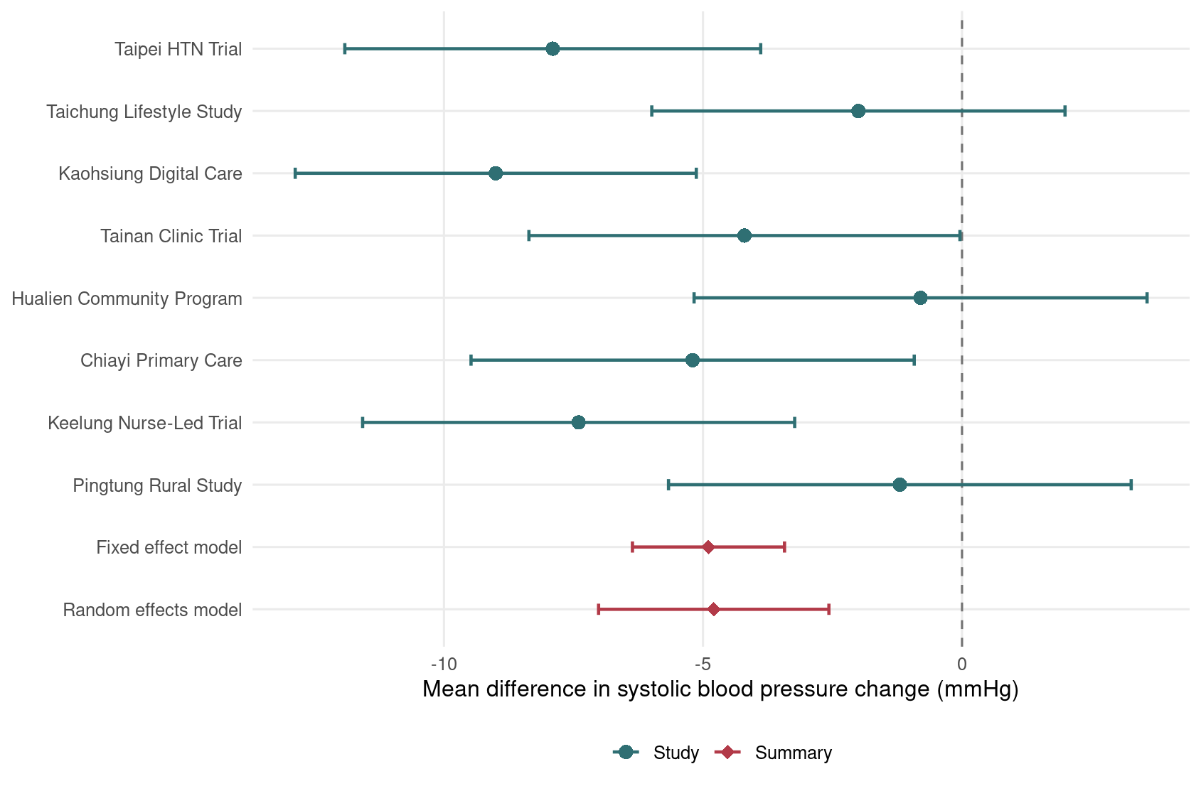
Figure 2.1: 高血壓照護介入對 12 週收縮壓變化的固定效應與隨機效應統合分析森林圖。
這張森林圖中,0 是無效果線 (line of no effect)。大多數研究點估計小於 0,表示介入組血壓下降較多;但各研究效果大小並不完全一致,因此隨機效應模型是合理的主要分析候選。
2.6 次族群分析
次族群分析 (subgroup analysis) 常用來探索異質性的可能來源。例如同樣是高血壓介入,在醫院、診所、社區場域的效果可能不同。這類分析最好事先在研究計畫書中定義,否則很容易變成「看哪個分組剛好顯著」的統計尋寶遊戲。
Code
subgroup_summary <- sbp_es |>
  group_by(setting) |>
  summarise(
    k = n(),
    theta = meta_iv(md, se_md)$random["theta"],
    lower = meta_iv(md, se_md)$random["lower"],
    upper = meta_iv(md, se_md)$random["upper"],
    tau2 = meta_iv(md, se_md)$tau2,
    .groups = "drop"
  )

kable(
  subgroup_summary,
  col.names = c("場域", "研究數", "隨機效應 MD", "95% CI 下限",
                "95% CI 上限", "tau-squared"),
  digits = 2
)
| Clinic |
2 |
-4.69 |
-7.67 |
-1.70 |
0 |
| Community |
3 |
-1.38 |
-3.84 |
1.08 |
0 |
| Hospital |
3 |
-8.14 |
-10.46 |
-5.82 |
0 |
Code
ggplot(subgroup_summary, aes(x = theta, y = setting)) +
  geom_vline(xintercept = 0, linetype = "dashed", color = "grey45") +
  geom_errorbar(
    aes(xmin = lower, xmax = upper),
    orientation = "y",
    width = 0.18,
    color = "#355C7D",
    linewidth = 0.9
  ) +
  geom_point(size = 3.5, color = "#C06C84") +
  labs(
    x = "Random-effects mean difference (mmHg)",
    y = NULL
  ) +
  theme_minimal(base_size = 12) +
  theme(panel.grid.minor = element_blank())
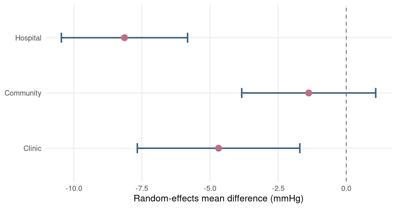
Figure 2.2: 依照照護場域分層的隨機效應平均差摘要。
此例暗示醫院場域的效果可能較大,社區場域較小。不過,每個次族群研究數很少,因此我們應把它視為探索性結果,而不是立即宣稱「醫院一定比較有效」。統計分析可以幫我們產生假說,但不能代替臨床與方法學判斷。
2.7 其他結局型態的統合分析
本章主要示範連續型結局,但臨床研究常見的效果量還包括存活結局、交叉試驗與調整後效果估計。
2.7.1 存活結局
存活結局 (survival outcome) 涉及事件發生時間,例如死亡、復發、住院或腎功能惡化。常用效果量是危險比 (hazard ratio, HR)。統合分析時通常使用 log(HR) 與其 SE:
Code
survival <- tibble::tibble(
  study = c("HF Follow-up Trial", "CKD Outcome Study", "Cardio-Renal Trial"),
  hr = c(0.82, 0.76, 0.88),
  ci_low = c(0.70, 0.61, 0.74),
  ci_high = c(0.96, 0.95, 1.05)
) |>
  mutate(
    log_hr = log(hr),
    se_log_hr = (log(ci_high) - log(ci_low)) / (2 * 1.96)
  )

kable(survival, digits = 3)
| HF Follow-up Trial |
0.82 |
0.70 |
0.96 |
-0.198 |
0.081 |
| CKD Outcome Study |
0.76 |
0.61 |
0.95 |
-0.274 |
0.113 |
| Cardio-Renal Trial |
0.88 |
0.74 |
1.05 |
-0.128 |
0.089 |
2.7.2 交叉試驗
交叉試驗 (cross-over trial) 中,同一位受試者會依序接受不同治療,因此兩個治療期間的結果具有相關性。若忽略此相關性,標準誤可能被估錯。理想資料是每位受試者的配對差異;若只有摘要資料,常需要知道配對相關係數 (within-person correlation) 或進行敏感度分析。
Code
crossover <- tibble::tibble(
  study = c("Crossover BP Trial A", "Crossover BP Trial B"),
  mean_difference = c(-3.2, -2.7),
  sd_paired_difference = c(8.1, 7.4),
  n = c(36, 42)
) |>
  mutate(se = sd_paired_difference / sqrt(n))

kable(crossover, digits = 2)
| Crossover BP Trial A |
-3.2 |
8.1 |
36 |
1.35 |
| Crossover BP Trial B |
-2.7 |
7.4 |
42 |
1.14 |
2.7.3 調整後治療效果
觀察性研究或非隨機研究常報告調整後效果估計 (adjusted treatment effect),例如調整年齡、性別、共病與基準風險後的平均差、勝算比或危險比。這類效果量通常以估計值加上 SE 或信賴區間進行 generic inverse-variance meta-analysis。
Code
adjusted <- tibble::tibble(
  study = c("Registry Analysis 1", "Claims-Based Study", "Hospital Cohort"),
  adjusted_md = c(-4.1, -2.9, -3.6),
  ci_low = c(-6.8, -5.1, -5.9),
  ci_high = c(-1.4, -0.7, -1.3)
) |>
  mutate(se = (ci_high - ci_low) / (2 * 1.96))

kable(adjusted, digits = 2)
| Registry Analysis 1 |
-4.1 |
-6.8 |
-1.4 |
1.38 |
| Claims-Based Study |
-2.9 |
-5.1 |
-0.7 |
1.12 |
| Hospital Cohort |
-3.6 |
-5.9 |
-1.3 |
1.17 |
這些例子共同指向同一個原則:只要能把每個研究轉成「效果估計 + 標準誤」,就可以使用反變異數架構進行統合分析。但效果量的可比性、調整變項是否一致、研究設計是否相近,仍然需要臨床與流行病學判斷。
2.8 R 工作流程與套件提醒
本章的完整 R 腳本儲存在 scripts/chapter2.R。你可以在專案根目錄執行:
Code
/usr/bin/Rscript scripts/chapter2.R
本章手動寫出核心公式,是為了讓你看懂模型背後的計算。正式分析時,建議使用成熟套件,例如 meta 或 metafor。目前本機已安裝這兩個套件;若你的環境尚未安裝,可用:
Code
install.packages(c("meta", "metafor"))
請記得,套件輸出不是統計神諭。你仍然要說明效果量選擇、模型選擇、異質性、敏感度分析與臨床可解釋性。R 可以幫你算得很快,但它不會替你負責任地解讀。
2.9 小結
本章從連續型結局開始,介紹 MD 與 SMD,接著比較固定效應與隨機效應模型。固定效應模型適合「研究共享同一真實效果」的情境;隨機效應模型則承認研究間可能存在真實差異。異質性不是麻煩的雜訊,而是研究脈絡給我們的訊息。
接下來的 Chapter 3 會把焦點轉到二元結局,正式處理勝算比、風險比、風險差、稀疏資料,以及 Mantel–Haenszel、Peto 等常見方法。簡單說,統合分析餐桌上的菜會越來越多,但我們會一盤一盤吃,不會把你丟進自助餐迷宮。
2.10 Glossary
| 連續型結局 |
continuous outcome |
| 平均差 |
mean difference, MD |
| 標準化平均差 |
standardised mean difference, SMD |
| 標準差 |
standard deviation, SD |
| 標準誤 |
standard error, SE |
| 固定效應模型 |
fixed-effect model |
| 隨機效應模型 |
random-effects model |
| 抽樣誤差 |
sampling error |
| 研究內變異 |
within-study variance |
| 反變異數權重 |
inverse-variance weight |
| 研究間變異 |
between-study variance |
| DerSimonian–Laird 方法 |
DerSimonian–Laird method |
| 限制最大概似法 |
restricted maximum likelihood, REML |
| Hartung–Knapp 調整 |
Hartung–Knapp adjustment |
| 預測區間 |
prediction interval |
| 異質性 |
heterogeneity |
| Cochran’s Q |
Cochran’s Q |
| I-squared |
I-squared, I2 |
| H-squared |
H-squared, H2 |
| tau-squared |
tau-squared, tau2 |
| 次族群分析 |
subgroup analysis |
| 無效果線 |
line of no effect |
| 存活結局 |
survival outcome |
| 危險比 |
hazard ratio, HR |
| 交叉試驗 |
cross-over trial |
| 配對相關係數 |
within-person correlation |
| 調整後效果估計 |
adjusted treatment effect |
| 通用反變異數統合分析 |
generic inverse-variance meta-analysis |