網路統合分析 (Network Meta-Analysis)

不只 A 比 B,也讓整個治療網絡一起說話

8.1 本章學習目標

讀完本章後,你應該能夠:

  1. 說明網絡統合分析 (network meta-analysis, NMA) 和傳統 pairwise meta-analysis 的差異。
  2. 解釋直接證據 (direct evidence)、間接證據 (indirect evidence)、一致性 (consistency) 與可傳遞性 (transitivity)。
  3. 使用 netmeta 套件進行固定效應與隨機效應 NMA。
  4. 繪製網絡圖 (network plot)、森林圖 (forest plot)、net heat plot 與 Bland–Altman 類圖。
  5. 解讀異質性與不一致性的 Q statistic decomposition。

前面章節多半在問:「A 治療和 B 治療相比如何?」但臨床決策常常更貪心,也更合理:A、B、C、D、E 全部放在一起,誰比較好?如果每一組都要直接做 head-to-head trial,研究經費大概會先哭出來。網絡統合分析就是為了解決這種多治療比較問題。

本章使用第二型糖尿病治療的教學範例,結局是 24 週達成 HbA1c 目標的比例。效果量是勝算比 (odds ratio, OR),OR > 1 代表相較於參考治療更可能達標。

8.2 網絡統合分析的概念與挑戰

網絡統合分析 (network meta-analysis) 可同時整合多種治療的直接與間接比較。直接證據 (direct evidence) 來自同一研究中直接比較兩個治療;間接證據 (indirect evidence) 則透過共同比較者連接。例如若有 A vs B 與 A vs C,我們就能間接推論 B vs C。

NMA 有兩個重要假設:

  • 可傳遞性 (transitivity):不同比較中的病人、研究設計與效果修飾因子足夠相似,使間接比較有意義。
  • 一致性 (consistency):直接證據與間接證據對同一比較的結論相容。

如果可傳遞性不合理,一致性檢定也救不了我們。這有點像拿不同科別、不同病人族群、不同追蹤時間的研究硬接成一張網:網是有了,但可能像臨時用膠帶黏的,不適合承重。

Code
arm_data <- tibble::tibble(
  studlab = c(
    "Taipei DPP4 Trial", "Taipei DPP4 Trial",
    "Taichung SGLT2 Trial", "Taichung SGLT2 Trial",
    "Kaohsiung GLP1 Trial", "Kaohsiung GLP1 Trial",
    "Tainan Active Comparator", "Tainan Active Comparator",
    "Hualien GLP1 Trial", "Hualien GLP1 Trial",
    "Chiayi Head-to-Head", "Chiayi Head-to-Head",
    "Keelung Insulin Trial", "Keelung Insulin Trial",
    "Pingtung Insulin Trial", "Pingtung Insulin Trial",
    "Miaoli SGLT2 Insulin", "Miaoli SGLT2 Insulin",
    "Yilan Three-Arm Trial", "Yilan Three-Arm Trial", "Yilan Three-Arm Trial",
    "Nantou Three-Arm Trial", "Nantou Three-Arm Trial", "Nantou Three-Arm Trial",
    "Taitung Three-Arm Trial", "Taitung Three-Arm Trial", "Taitung Three-Arm Trial",
    "Yunlin DPP4 Trial", "Yunlin DPP4 Trial",
    "Penghu Insulin Trial", "Penghu Insulin Trial"
  ),
  treat = c(
    "Usual care", "DPP-4 inhibitor",
    "Usual care", "SGLT2 inhibitor",
    "Usual care", "GLP-1 RA",
    "DPP-4 inhibitor", "SGLT2 inhibitor",
    "DPP-4 inhibitor", "GLP-1 RA",
    "SGLT2 inhibitor", "GLP-1 RA",
    "Usual care", "Basal insulin",
    "DPP-4 inhibitor", "Basal insulin",
    "SGLT2 inhibitor", "Basal insulin",
    "Usual care", "DPP-4 inhibitor", "SGLT2 inhibitor",
    "Usual care", "GLP-1 RA", "SGLT2 inhibitor",
    "DPP-4 inhibitor", "GLP-1 RA", "Basal insulin",
    "Usual care", "DPP-4 inhibitor",
    "Usual care", "Basal insulin"
  ),
  event = c(
    42, 58,
    45, 82,
    50, 94,
    62, 85,
    65, 90,
    88, 95,
    38, 70,
    56, 78,
    80, 76,
    40, 55, 75,
    44, 82, 77,
    58, 72, 66,
    35, 49,
    43, 74
  ),
  n = c(
    220, 218,
    240, 238,
    260, 258,
    230, 232,
    250, 248,
    245, 244,
    180, 178,
    210, 212,
    220, 218,
    200, 198, 202,
    210, 212, 208,
    190, 188, 186,
    170, 168,
    205, 204
  )
) |>
  mutate(non_event = n - event)

kable(
  arm_data,
  col.names = c("研究", "治療", "達標人數", "總人數", "未達標人數"),
  digits = 0
)
研究 治療 達標人數 總人數 未達標人數
Taipei DPP4 Trial Usual care 42 220 178
Taipei DPP4 Trial DPP-4 inhibitor 58 218 160
Taichung SGLT2 Trial Usual care 45 240 195
Taichung SGLT2 Trial SGLT2 inhibitor 82 238 156
Kaohsiung GLP1 Trial Usual care 50 260 210
Kaohsiung GLP1 Trial GLP-1 RA 94 258 164
Tainan Active Comparator DPP-4 inhibitor 62 230 168
Tainan Active Comparator SGLT2 inhibitor 85 232 147
Hualien GLP1 Trial DPP-4 inhibitor 65 250 185
Hualien GLP1 Trial GLP-1 RA 90 248 158
Chiayi Head-to-Head SGLT2 inhibitor 88 245 157
Chiayi Head-to-Head GLP-1 RA 95 244 149
Keelung Insulin Trial Usual care 38 180 142
Keelung Insulin Trial Basal insulin 70 178 108
Pingtung Insulin Trial DPP-4 inhibitor 56 210 154
Pingtung Insulin Trial Basal insulin 78 212 134
Miaoli SGLT2 Insulin SGLT2 inhibitor 80 220 140
Miaoli SGLT2 Insulin Basal insulin 76 218 142
Yilan Three-Arm Trial Usual care 40 200 160
Yilan Three-Arm Trial DPP-4 inhibitor 55 198 143
Yilan Three-Arm Trial SGLT2 inhibitor 75 202 127
Nantou Three-Arm Trial Usual care 44 210 166
Nantou Three-Arm Trial GLP-1 RA 82 212 130
Nantou Three-Arm Trial SGLT2 inhibitor 77 208 131
Taitung Three-Arm Trial DPP-4 inhibitor 58 190 132
Taitung Three-Arm Trial GLP-1 RA 72 188 116
Taitung Three-Arm Trial Basal insulin 66 186 120
Yunlin DPP4 Trial Usual care 35 170 135
Yunlin DPP4 Trial DPP-4 inhibitor 49 168 119
Penghu Insulin Trial Usual care 43 205 162
Penghu Insulin Trial Basal insulin 74 204 130

8.3 模型與估計

NMA 可用不同架構估計。本章使用 frequentist graph-theoretical approach,也就是 netmeta 套件的主要方法。對二元結局,我們先用 pairwise() 把 arm-based 資料轉為 study-level treatment contrasts。

Code
pw <- pairwise(
  treat = treat,
  event = event,
  n = n,
  studlab = studlab,
  data = arm_data,
  sm = "OR"
)

kable(
  pw |>
    transmute(研究 = studlab, 治療1 = treat1, 治療2 = treat2,
              `log OR` = TE, `SE` = seTE),
  digits = 3
)
研究 治療1 治療2 log OR SE
Taipei DPP4 Trial Usual care DPP-4 inhibitor -0.429 0.230
Taichung SGLT2 Trial Usual care SGLT2 inhibitor -0.823 0.214
Kaohsiung GLP1 Trial Usual care GLP-1 RA -0.879 0.204
Tainan Active Comparator DPP-4 inhibitor SGLT2 inhibitor -0.449 0.202
Hualien GLP1 Trial DPP-4 inhibitor GLP-1 RA -0.483 0.196
Chiayi Head-to-Head SGLT2 inhibitor GLP-1 RA -0.129 0.187
Keelung Insulin Trial Usual care Basal insulin -0.885 0.239
Pingtung Insulin Trial DPP-4 inhibitor Basal insulin -0.470 0.211
Miaoli SGLT2 Insulin SGLT2 inhibitor Basal insulin 0.065 0.200
Yilan Three-Arm Trial Usual care DPP-4 inhibitor -0.431 0.238
Yilan Three-Arm Trial Usual care SGLT2 inhibitor -0.860 0.229
Yilan Three-Arm Trial DPP-4 inhibitor SGLT2 inhibitor -0.429 0.215
Nantou Three-Arm Trial Usual care GLP-1 RA -0.867 0.221
Nantou Three-Arm Trial Usual care SGLT2 inhibitor -0.796 0.222
Nantou Three-Arm Trial GLP-1 RA SGLT2 inhibitor 0.071 0.201
Taitung Three-Arm Trial DPP-4 inhibitor Basal insulin -0.225 0.220
Taitung Three-Arm Trial DPP-4 inhibitor GLP-1 RA -0.345 0.218
Taitung Three-Arm Trial GLP-1 RA Basal insulin 0.121 0.214
Yunlin DPP4 Trial Usual care DPP-4 inhibitor -0.463 0.255
Penghu Insulin Trial Usual care Basal insulin -0.763 0.225

8.3.1 固定效應模型

固定效應 NMA (fixed effect network meta-analysis) 假設每個治療比較只有一個共同真實效果,研究差異來自抽樣誤差。

Code
nma_common <- netmeta(
  TE,
  seTE,
  treat1,
  treat2,
  studlab,
  data = pw,
  sm = "OR",
  reference.group = "Usual care",
  common = TRUE,
  random = FALSE,
  small.values = "bad"
)

print(nma_common)
Number of studies: k = 14
Number of pairwise comparisons: m = 20
Number of treatments: n = 5
Number of designs: d = 12

Common effects model

Treatment estimate (other treatments vs 'Usual care'):
                    OR           95% CI    z  p-value
Basal insulin   2.2240 [1.7977; 2.7515] 7.36 < 0.0001
DPP-4 inhibitor 1.5375 [1.2692; 1.8626] 4.40 < 0.0001
GLP-1 RA        2.4564 [2.0058; 3.0082] 8.69 < 0.0001
SGLT2 inhibitor 2.3018 [1.9003; 2.7882] 8.52 < 0.0001
Usual care           .                .    .        .

Quantifying heterogeneity / inconsistency:
tau^2 = 0; tau = 0; I^2 = 0% [0.0%; 55.0%]

Tests of heterogeneity (within designs) and inconsistency (between designs):
                   Q d.f. p-value
Total           1.16   13  1.0000
Within designs  0.15    2  0.9291
Between designs 1.01   11  0.9999

Details of network meta-analysis methods:
- Frequentist graph-theoretical approach
- DerSimonian-Laird estimator for tau^2
- Calculation of I^2 based on Q

8.3.2 隨機效應模型

隨機效應 NMA (random effects network meta-analysis) 承認不同研究對同一比較可能有不同真實效果,並估計共同的研究間變異 \(\tau^2\)

Code
nma_random <- netmeta(
  TE,
  seTE,
  treat1,
  treat2,
  studlab,
  data = pw,
  sm = "OR",
  reference.group = "Usual care",
  common = TRUE,
  random = TRUE,
  method.tau = "DL",
  small.values = "bad"
)

print(nma_random)
Number of studies: k = 14
Number of pairwise comparisons: m = 20
Number of treatments: n = 5
Number of designs: d = 12

Common effects model

Treatment estimate (other treatments vs 'Usual care'):
                    OR           95% CI    z  p-value
Basal insulin   2.2240 [1.7977; 2.7515] 7.36 < 0.0001
DPP-4 inhibitor 1.5375 [1.2692; 1.8626] 4.40 < 0.0001
GLP-1 RA        2.4564 [2.0058; 3.0082] 8.69 < 0.0001
SGLT2 inhibitor 2.3018 [1.9003; 2.7882] 8.52 < 0.0001
Usual care           .                .    .        .

Random effects model

Treatment estimate (other treatments vs 'Usual care'):
                    OR           95% CI    z  p-value
Basal insulin   2.2240 [1.7977; 2.7515] 7.36 < 0.0001
DPP-4 inhibitor 1.5375 [1.2692; 1.8626] 4.40 < 0.0001
GLP-1 RA        2.4564 [2.0058; 3.0082] 8.69 < 0.0001
SGLT2 inhibitor 2.3018 [1.9003; 2.7882] 8.52 < 0.0001
Usual care           .                .    .        .

Quantifying heterogeneity / inconsistency:
tau^2 = 0; tau = 0; I^2 = 0% [0.0%; 55.0%]

Tests of heterogeneity (within designs) and inconsistency (between designs):
                   Q d.f. p-value
Total           1.16   13  1.0000
Within designs  0.15    2  0.9291
Between designs 1.01   11  0.9999

Details of network meta-analysis methods:
- Frequentist graph-theoretical approach
- DerSimonian-Laird estimator for tau^2
- Calculation of I^2 based on Q

8.4 使用 netmeta 進行網絡統合分析

8.4.1 基本分析與網絡圖

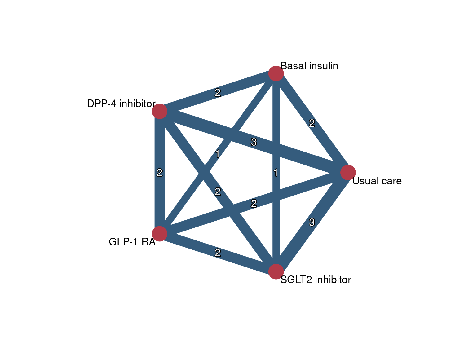
網絡圖 (network plot) 顯示哪些治療有直接比較。節點代表治療,線代表至少一個研究直接比較兩治療。線越粗,通常表示研究數越多。

Code
netgraph(
  nma_random,
  plastic = FALSE,
  points = TRUE,
  cex.points = 5,
  thickness = "number.of.studies",
  number.of.studies = TRUE,
  col = "#355C7D",
  col.points = "#B23A48",
  bg.points = "#B23A48",
  cex = 1.05
)

Figure 8.1: 第二型糖尿病治療達成 HbA1c 目標的治療網絡圖。

8.4.2 更詳細檢視輸出

netmeta 輸出包含治療數、比較數、設計數、common/random effects results、異質性與不一致性檢定。NMA 的輸出比傳統統合分析熱鬧一些,第一次看會像進到大型醫院地下街,方向很多但不要慌。

Code
ref <- "Usual care"
treatments <- setdiff(nma_random$trts, ref)
summary_vs_ref <- tibble::tibble(
  treatment = treatments,
  log_or = sapply(treatments, function(x) nma_random$TE.random[x, ref]),
  lower = sapply(treatments, function(x) nma_random$lower.random[x, ref]),
  upper = sapply(treatments, function(x) nma_random$upper.random[x, ref])
) |>
  mutate(
    or = exp(log_or),
    or_low = exp(lower),
    or_high = exp(upper),
    treatment = factor(treatment, levels = treatment[order(or)])
  )

kable(
  summary_vs_ref |>
    transmute(治療 = treatment, `OR vs usual care` = or,
              `95% CI` = sprintf("%.2f to %.2f", or_low, or_high)),
  digits = 3
)
治療 OR vs usual care 95% CI
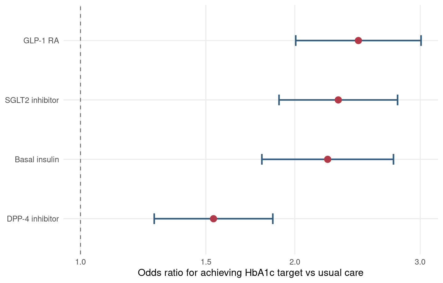
Basal insulin 2.224 1.80 to 2.75
DPP-4 inhibitor 1.538 1.27 to 1.86
GLP-1 RA 2.456 2.01 to 3.01
SGLT2 inhibitor 2.302 1.90 to 2.79

8.4.3 排名與 P-score

治療排名常用 P-score 或 SUCRA 類指標呈現。請小心:排名不是臨床建議。若兩個治療效果差異很小,排名第一與第二可能只是統計座位表,不是勝負判決。

Code
ranking <- netrank(nma_random, small.values = "bad")$Pscore.random |>
  as.data.frame() |>
  tibble::rownames_to_column("treatment") |>
  setNames(c("treatment", "pscore")) |>
  arrange(desc(pscore))

kable(ranking, col.names = c("治療", "P-score"), digits = 3)
治療 P-score
GLP-1 RA 0.884
SGLT2 inhibitor 0.720
Basal insulin 0.646
DPP-4 inhibitor 0.250
Usual care 0.000

8.4.4 森林圖

Code
ggplot(summary_vs_ref, aes(x = or, y = treatment)) +
  geom_vline(xintercept = 1, linetype = "dashed", color = "grey45") +
  geom_errorbar(aes(xmin = or_low, xmax = or_high), orientation = "y",
                width = 0.18, color = "#355C7D", linewidth = 0.9) +
  geom_point(size = 3.4, color = "#B23A48") +
  scale_x_log10(breaks = c(0.75, 1, 1.5, 2, 3, 4)) +
  labs(x = "Odds ratio for achieving HbA1c target vs usual care",
       y = NULL) +
  theme_minimal(base_size = 12) +
  theme(panel.grid.minor = element_blank())

Figure 8.2: 隨機效應 NMA 中各治療相對於 usual care 的 OR 森林圖。

8.5 異質性統計量的分解

NMA 可將 Q statistic 分解為總變異、within-design heterogeneity 與 between-design inconsistency。Within-design heterogeneity 類似傳統統合分析中的異質性;between-design inconsistency 則反映不同設計提供的證據是否一致。

Code
q_summary <- tibble::tibble(
  component = c("Total", "Within designs", "Between designs"),
  q = c(nma_random$Q, nma_random$Q.heterogeneity, nma_random$Q.inconsistency),
  df = c(nma_random$df.Q, nma_random$df.Q.heterogeneity, nma_random$df.Q.inconsistency),
  p_value = c(nma_random$pval.Q, nma_random$pval.Q.heterogeneity, nma_random$pval.Q.inconsistency)
)

kable(q_summary, col.names = c("成分", "Q", "df", "p 值"), digits = 3)
成分 Q df p 值
Total 1.162 13 1.000
Within designs 0.147 2 0.929
Between designs 1.015 11 1.000
Code
kable(nma_random$Q.decomp, digits = 3)
treat1 treat2 Q df pval.Q
Basal insulin DPP-4 inhibitor 0.509 1 0.476
Basal insulin GLP-1 RA 0.000 0 NA
Basal insulin SGLT2 inhibitor 0.000 0 NA
Basal insulin Usual care 0.138 1 0.711
DPP-4 inhibitor GLP-1 RA 0.174 1 0.677
DPP-4 inhibitor SGLT2 inhibitor 0.004 1 0.950
DPP-4 inhibitor Usual care 0.011 2 0.995
GLP-1 RA SGLT2 inhibitor 0.038 1 0.846
GLP-1 RA Usual care 0.001 1 0.973
SGLT2 inhibitor Usual care 0.026 2 0.987

如果 between-design inconsistency 很明顯,就要回頭檢查 transitivity:不同比較的族群是否類似?基準 HbA1c、疾病期間、背景用藥、腎功能、追蹤時間是否相近?統計檢定是警報器,不是偵探本身。

8.6 Net heat plot

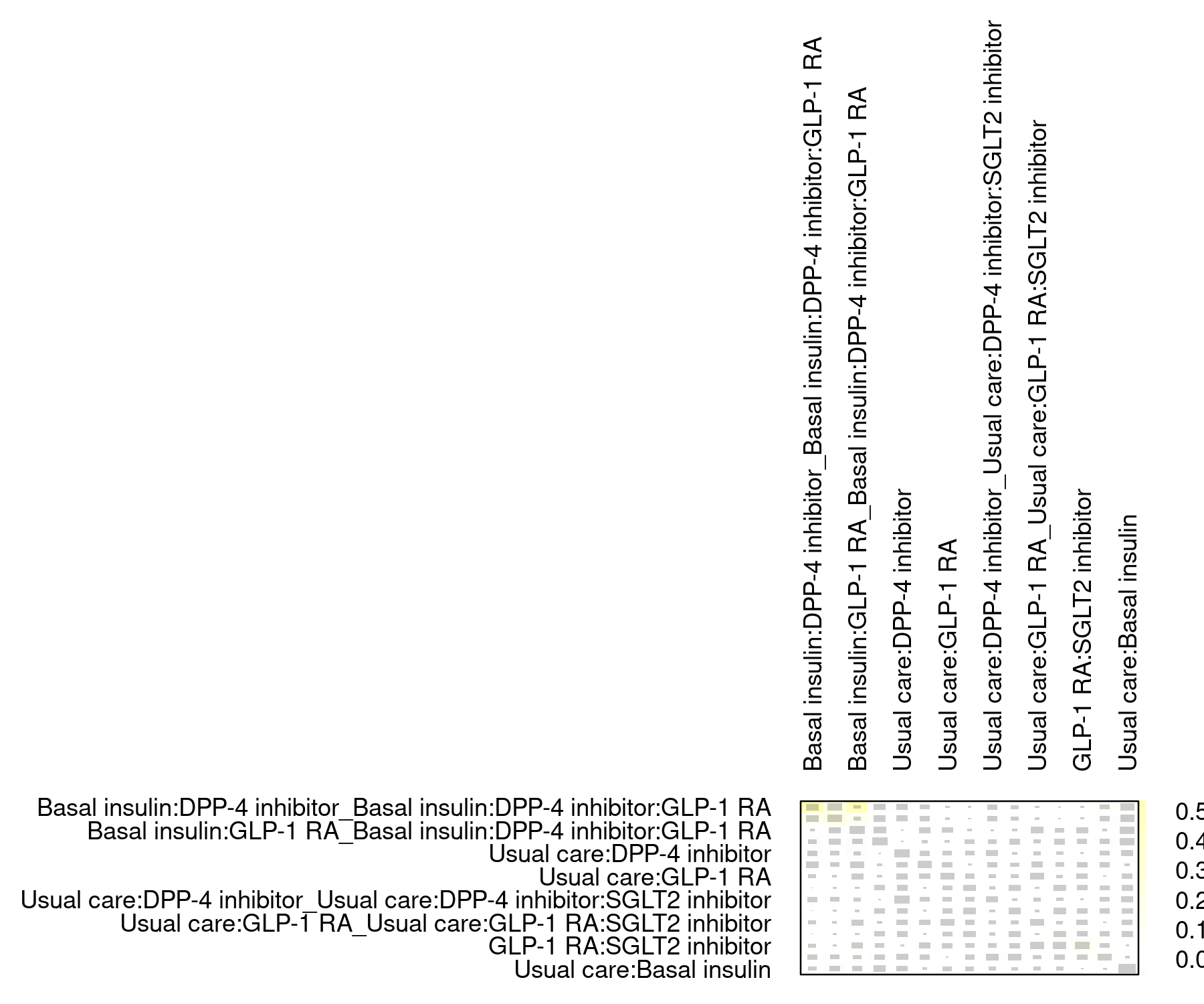
Net heat plot 用顏色顯示每個直接比較對網絡不一致性的貢獻。顏色越熱,代表該比較越值得進一步檢查。它不是叫你刪研究,而是叫你回去讀研究。

Code
netheat(nma_random)

Figure 8.3: Net heat plot 用於檢視直接比較對不一致性的貢獻。

8.6.1 Bland–Altman 圖:檢視異質性對治療比較的影響

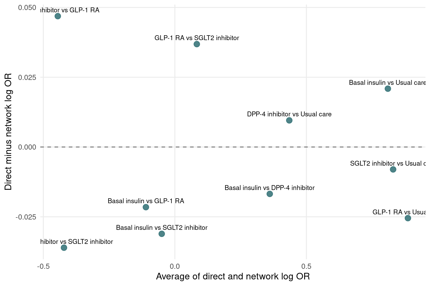
Bland–Altman 類圖可用來比較直接估計與整體網絡估計。若差異集中在 0 附近,代表直接與網絡估計大致相容;若某些比較明顯偏離,則值得檢查。

Code
direct_network <- expand.grid(
  treat1 = nma_random$trts,
  treat2 = nma_random$trts,
  stringsAsFactors = FALSE
) |>
  filter(treat1 < treat2) |>
  rowwise() |>
  mutate(
    direct = nma_random$TE.direct.random[treat1, treat2],
    network = nma_random$TE.random[treat1, treat2],
    average = (direct + network) / 2,
    difference = direct - network
  ) |>
  ungroup() |>
  filter(!is.na(direct), !is.na(network))

ggplot(direct_network, aes(x = average, y = difference)) +
  geom_hline(yintercept = 0, linetype = "dashed", color = "grey45") +
  geom_point(size = 3.2, color = "#2F6F73", alpha = 0.85) +
  geom_text(aes(label = paste(treat1, "vs", treat2)), vjust = -0.8, size = 3) +
  labs(x = "Average of direct and network log OR",
       y = "Direct minus network log OR") +
  theme_minimal(base_size = 12) +
  theme(panel.grid.minor = element_blank())

Figure 8.4: 直接估計與網絡估計的 Bland–Altman 類比較圖。

8.7 R 工作流程與套件提醒

本章完整 R 腳本儲存在 scripts/chapter8.R。你可以在專案根目錄執行:

Code
/usr/bin/Rscript scripts/chapter8.R

本章使用 netmetametaggplot2dplyrknitr,目前本機皆已安裝。若你的環境尚未安裝,可執行:

Code
install.packages(c("netmeta", "meta"))

8.8 小結

網絡統合分析讓我們能同時比較多個治療,整合直接與間接證據。它的威力很大,但假設也更重:transitivity 與 consistency 必須被認真檢查。網絡圖告訴我們證據結構,森林圖呈現相對效果,ranking 提供排序線索,Q decomposition 與 net heat plot 幫助檢視異質性與不一致性。

下一章會轉向診斷準確度研究的統合分析。診斷研究會帶來敏感度、特異度與 ROC curve 等新角色;統計舞台會換布景,但我們仍然會用同一個原則:先理解資料,再選模型。

8.9 Glossary

中文 English
網絡統合分析 network meta-analysis, NMA
傳統兩兩統合分析 pairwise meta-analysis
直接證據 direct evidence
間接證據 indirect evidence
一致性 consistency
可傳遞性 transitivity
網絡圖 network plot
森林圖 forest plot
勝算比 odds ratio, OR
固定效應網絡統合分析 fixed effect network meta-analysis
隨機效應網絡統合分析 random effects network meta-analysis
研究間變異 between-study variance
P-score P-score
SUCRA surface under the cumulative ranking curve, SUCRA
Q statistic decomposition Q statistic decomposition
Within-design heterogeneity within-design heterogeneity
Between-design inconsistency between-design inconsistency
Net heat plot net heat plot
Bland–Altman 圖 Bland–Altman plot