3.1 本章學習目標
讀完本章後,你應該能夠:
- 說明二元結局 (binary outcome) 在臨床研究中的資料結構。
- 計算並解讀勝算比 (odds ratio, OR)、風險比 (risk ratio, RR)、風險差 (risk difference, RD) 與 arcsine 差異 (arcsine difference)。
- 理解稀疏資料 (sparse data) 與零事件 (zero event) 對統合分析的影響。
- 比較反變異數法 (inverse-variance method)、Mantel–Haenszel 方法 (Mantel–Haenszel method) 與 Peto 方法 (Peto method)。
- 使用固定效應模型與隨機效應模型分析二元結局,並進行基本異質性與次族群分析。
二元結局在醫學研究中非常常見:感染或未感染、死亡或存活、復發或未復發、是否發生重大不良事件。它直覺、臨床上好懂,但統計上有時比看起來更調皮。尤其當事件很少時,一個 0 就可能讓 OR 公式當場臉色發白。
本章使用一個臨床情境貫穿:圍手術期抗生素是否能降低手術部位感染 (surgical site infection, SSI)。每篇研究都可以整理成 2x2 表:介入組與對照組,各自有多少人發生感染。
3.2 二元結局的資料結構
二元結局通常整理成下列表格:
| 介入組 |
\(a\) |
\(b\) |
| 對照組 |
\(c\) |
\(d\) |
其中介入組總人數是 \(n_1=a+b\),對照組總人數是 \(n_0=c+d\)。以下是本章的教學資料:8 個隨機對照試驗比較圍手術期抗生素與標準照護對 SSI 的影響。
Code
ci_norm <- function(theta, se, level = 0.95) {
  z <- qnorm(1 - (1 - level) / 2)
  c(lower = theta - z * se, upper = theta + z * se)
}

meta_iv <- function(yi, sei) {
  vi <- sei^2
  k <- length(yi)
  w_fe <- 1 / vi
  theta_fe <- sum(w_fe * yi) / sum(w_fe)
  se_fe <- sqrt(1 / sum(w_fe))
  q <- sum(w_fe * (yi - theta_fe)^2)
  df <- k - 1
  c_dl <- sum(w_fe) - sum(w_fe^2) / sum(w_fe)
  tau2 <- max(0, (q - df) / c_dl)
  w_re <- 1 / (vi + tau2)
  theta_re <- sum(w_re * yi) / sum(w_re)
  se_re <- sqrt(1 / sum(w_re))
  list(
    fixed = c(theta = theta_fe, se = se_fe, ci_norm(theta_fe, se_fe)),
    random = c(theta = theta_re, se = se_re, ci_norm(theta_re, se_re)),
    q = q,
    df = df,
    p_q = pchisq(q, df, lower.tail = FALSE),
    tau2 = tau2,
    tau = sqrt(tau2),
    i2 = max(0, (q - df) / q) * 100
  )
}

binary_effects <- function(dat, correction = 0) {
  dat |>
    mutate(
      a = event_tx + correction,
      b = total_tx - event_tx + correction,
      c = event_ctrl + correction,
      d = total_ctrl - event_ctrl + correction,
      n1 = a + b,
      n0 = c + d,
      p1 = a / n1,
      p0 = c / n0,
      log_or = log((a * d) / (b * c)),
      se_log_or = sqrt(1 / a + 1 / b + 1 / c + 1 / d),
      or = exp(log_or),
      or_low = exp(log_or - 1.96 * se_log_or),
      or_high = exp(log_or + 1.96 * se_log_or),
      log_rr = log(p1 / p0),
      se_log_rr = sqrt(1 / a - 1 / n1 + 1 / c - 1 / n0),
      rr = exp(log_rr),
      rr_low = exp(log_rr - 1.96 * se_log_rr),
      rr_high = exp(log_rr + 1.96 * se_log_rr),
      rd = p1 - p0,
      se_rd = sqrt(p1 * (1 - p1) / n1 + p0 * (1 - p0) / n0),
      rd_low = rd - 1.96 * se_rd,
      rd_high = rd + 1.96 * se_rd,
      arcsine_diff = asin(sqrt(p1)) - asin(sqrt(p0)),
      se_arcsine = sqrt(1 / (4 * n1) + 1 / (4 * n0))
    )
}

peto_or <- function(dat) {
  peto_dat <- dat |>
    mutate(
      n1 = total_tx,
      n0 = total_ctrl,
      n = n1 + n0,
      m = event_tx + event_ctrl,
      expected_tx = n1 * m / n,
      oe = event_tx - expected_tx,
      v = n1 * n0 * m * (n - m) / (n^2 * (n - 1))
    )

  log_or <- sum(peto_dat$oe) / sum(peto_dat$v)
  se <- sqrt(1 / sum(peto_dat$v))
  list(
    study = peto_dat,
    pooled = c(
      log_or = log_or,
      se = se,
      lower = log_or - 1.96 * se,
      upper = log_or + 1.96 * se
    )
  )
}
Code
ssi <- tibble::tibble(
  study = c("Taipei Surgery Trial", "Taichung OR Study",
            "Kaohsiung Abdominal Trial", "Tainan Clean-Contaminated Trial",
            "Hualien Surgical Care", "Chiayi Colorectal Trial",
            "Keelung Perioperative Trial", "Pingtung Hospital Study"),
  setting = c("Clean-contaminated", "Clean-contaminated", "Colorectal",
              "Clean-contaminated", "Contaminated", "Colorectal",
              "Clean-contaminated", "Contaminated"),
  event_tx = c(12, 18, 28, 10, 32, 31, 14, 30),
  total_tx = c(310, 360, 280, 250, 260, 300, 290, 240),
  event_ctrl = c(25, 34, 39, 22, 28, 45, 30, 26),
  total_ctrl = c(305, 355, 275, 248, 255, 295, 285, 238)
)

kable(
  ssi,
  col.names = c("研究", "手術傷口類型", "抗生素組感染數", "抗生素組總人數",
                "對照組感染數", "對照組總人數"),
  digits = 0
)
| Taipei Surgery Trial |
Clean-contaminated |
12 |
310 |
25 |
305 |
| Taichung OR Study |
Clean-contaminated |
18 |
360 |
34 |
355 |
| Kaohsiung Abdominal Trial |
Colorectal |
28 |
280 |
39 |
275 |
| Tainan Clean-Contaminated Trial |
Clean-contaminated |
10 |
250 |
22 |
248 |
| Hualien Surgical Care |
Contaminated |
32 |
260 |
28 |
255 |
| Chiayi Colorectal Trial |
Colorectal |
31 |
300 |
45 |
295 |
| Keelung Perioperative Trial |
Clean-contaminated |
14 |
290 |
30 |
285 |
| Pingtung Hospital Study |
Contaminated |
30 |
240 |
26 |
238 |
3.3 二元結局的效果量
3.3.1 勝算比
勝算比 (odds ratio, OR) 比較兩組事件勝算 (odds) 的比例:
\[
OR = \frac{a/b}{c/d} = \frac{ad}{bc}
\]
若 OR < 1,代表介入組事件勝算較低;若 OR > 1,代表介入組事件勝算較高。OR 常用於病例對照研究與 logistic regression,也常出現在二元結局的統合分析。
Code
ssi_es <- binary_effects(ssi)

kable(
  ssi_es |>
    transmute(
      研究 = study,
      `OR` = or,
      `OR 95% CI` = sprintf("%.2f to %.2f", or_low, or_high),
      `RR` = rr,
      `RD` = rd,
      `Arcsine difference` = arcsine_diff
    ),
  digits = 3
)
| Taipei Surgery Trial |
0.451 |
0.22 to 0.91 |
0.472 |
-0.043 |
-0.092 |
| Taichung OR Study |
0.497 |
0.28 to 0.90 |
0.522 |
-0.046 |
-0.089 |
| Kaohsiung Abdominal Trial |
0.672 |
0.40 to 1.13 |
0.705 |
-0.042 |
-0.064 |
| Tainan Clean-Contaminated Trial |
0.428 |
0.20 to 0.92 |
0.451 |
-0.049 |
-0.101 |
| Hualien Surgical Care |
1.138 |
0.66 to 1.95 |
1.121 |
0.013 |
0.021 |
| Chiayi Colorectal Trial |
0.640 |
0.39 to 1.04 |
0.677 |
-0.049 |
-0.074 |
| Keelung Perioperative Trial |
0.431 |
0.22 to 0.83 |
0.459 |
-0.057 |
-0.109 |
| Pingtung Hospital Study |
1.165 |
0.67 to 2.04 |
1.144 |
0.016 |
0.025 |
OR 的優點是數學性質好,尤其適合 logistic 模型;缺點是當事件不罕見時,OR 可能比 RR 看起來更誇張。這不是 OR 壞心眼,而是它描述的是勝算,不是風險。
3.3.2 風險比
風險比 (risk ratio, RR) 比較兩組事件風險:
\[
RR = \frac{a/(a+b)}{c/(c+d)}
\]
RR 對臨床讀者通常更直覺。若 SSI 風險從 10% 降到 5%,RR 是 0.50,意思是風險約減半。
3.3.3 風險差
風險差 (risk difference, RD) 是兩組絕對風險差:
\[
RD = \frac{a}{a+b} - \frac{c}{c+d}
\]
RD 的臨床意義很強,因為它能連到需治數 (number needed to treat, NNT)。若 RD = -0.04,代表每 100 位病人約可少 4 位發生 SSI,NNT 約為 \(1/0.04=25\)。
3.3.4 Arcsine 差異
Arcsine 差異 (arcsine difference) 是用事件比例的平方根 arcsine 轉換來衡量差異:
\[
ASD = \arcsin(\sqrt{p_1}) - \arcsin(\sqrt{p_0})
\]
它在事件很少或比例接近 0/1 時有些數學優點,但臨床解讀比較不直覺。實務上,讀者看到 arcsine 差異可能會問:「這能換成感染少幾個人嗎?」這個問題非常合理。
3.4 稀疏資料與零事件
稀疏資料 (sparse data) 指事件數很少的情況。若某研究某一組事件數為 0,OR 或 RR 的公式可能會出現除以 0。常見處理方式包括連續性校正 (continuity correction),例如在每個 cell 加上 0.5。不過校正會影響估計,尤其小研究很多時更明顯。
Code
sparse <- tibble::tibble(
  study = c("Rare Bleeding Trial A", "Rare Bleeding Trial B",
            "Rare Bleeding Trial C", "Rare Bleeding Trial D"),
  event_tx = c(0, 1, 0, 2),
  total_tx = c(120, 95, 140, 110),
  event_ctrl = c(2, 1, 0, 3),
  total_ctrl = c(118, 97, 138, 112)
)

sparse_cc <- binary_effects(sparse, correction = 0.5)

kable(
  sparse_cc |>
    transmute(
      研究 = study,
      `校正後 OR` = or,
      `95% CI` = sprintf("%.2f to %.2f", or_low, or_high),
      `校正後 RR` = rr
    ),
  digits = 3
)
| Rare Bleeding Trial A |
0.193 |
0.01 to 4.07 |
0.197 |
| Rare Bleeding Trial B |
1.021 |
0.10 to 9.99 |
1.021 |
| Rare Bleeding Trial C |
0.986 |
0.02 to 50.03 |
0.986 |
| Rare Bleeding Trial D |
0.721 |
0.14 to 3.73 |
0.727 |
若兩組都沒有事件,該研究對相對效果通常提供很少資訊,但對絕對風險仍有描述價值。稀疏資料分析沒有一招走天下,必須同時考慮事件率、治療效果大小、組間平衡、研究數量與模型假設。
3.4.1 Peto 勝算比
Peto 勝算比 (Peto odds ratio) 是稀有事件固定效應分析常見方法之一。它使用每個研究的觀察事件數減期望事件數 (observed minus expected, O-E) 與其變異數 \(V\):
\[
\log(OR_{Peto}) = \frac{\sum(O-E)}{\sum V}
\]
Peto 方法在事件稀少、治療效果不太大、組間樣本數平衡時表現較好;若治療效果很大或組間嚴重不平衡,就要小心。
Code
sparse_peto <- peto_or(sparse)

kable(
  sparse_peto$study |>
    transmute(
      研究 = study,
      `O-E` = oe,
      `V` = v
    ),
  digits = 3
)
| Rare Bleeding Trial A |
-1.008 |
0.498 |
| Rare Bleeding Trial B |
0.010 |
0.497 |
| Rare Bleeding Trial C |
0.000 |
0.000 |
| Rare Bleeding Trial D |
-0.477 |
1.227 |
Code
kable(
  tibble::tibble(
    method = "Peto OR",
    estimate = exp(sparse_peto$pooled["log_or"]),
    lower = exp(sparse_peto$pooled["lower"]),
    upper = exp(sparse_peto$pooled["upper"])
  ),
  col.names = c("方法", "OR", "95% CI 下限", "95% CI 上限"),
  digits = 3
)
| Peto OR |
0.515 |
0.138 |
1.917 |
3.5 固定效應模型
3.5.1 反變異數法
反變異數法 (inverse-variance method) 先把 OR 或 RR 轉成對數尺度,再用標準誤計算權重。以 OR 為例:
\[
\log(OR_i) = \log\left(\frac{a_id_i}{b_ic_i}\right)
\]
\[
SE\{\log(OR_i)\} = \sqrt{\frac{1}{a_i}+\frac{1}{b_i}+\frac{1}{c_i}+\frac{1}{d_i}}
\]
Code
or_meta <- meta_iv(ssi_es$log_or, ssi_es$se_log_or)
rr_meta <- meta_iv(ssi_es$log_rr, ssi_es$se_log_rr)
rd_meta <- meta_iv(ssi_es$rd, ssi_es$se_rd)

iv_tbl <- tibble::tibble(
  effect = c("Odds ratio", "Risk ratio", "Risk difference"),
  estimate = c(exp(or_meta$fixed["theta"]), exp(rr_meta$fixed["theta"]),
               rd_meta$fixed["theta"]),
  lower = c(exp(or_meta$fixed["lower"]), exp(rr_meta$fixed["lower"]),
            rd_meta$fixed["lower"]),
  upper = c(exp(or_meta$fixed["upper"]), exp(rr_meta$fixed["upper"]),
            rd_meta$fixed["upper"])
)

kable(
  iv_tbl,
  col.names = c("效果量", "固定效應估計", "95% CI 下限", "95% CI 上限"),
  digits = 3
)
| Odds ratio |
0.670 |
0.545 |
0.823 |
| Risk ratio |
0.704 |
0.584 |
0.848 |
| Risk difference |
-0.037 |
-0.054 |
-0.021 |
在這個例子中,OR 與 RR 都小於 1,表示圍手術期抗生素可降低 SSI。RD 則提供絕對風險差,對病人溝通與政策評估特別有幫助。
3.5.2 Mantel–Haenszel 方法
Mantel–Haenszel 方法 (Mantel–Haenszel method) 是二元結局固定效應統合分析的經典方法,尤其適合事件率不高且研究數有限的情境。R 的 base package 內建 mantelhaen.test(),可以對分層 2x2 表估計共同 OR。
Code
mh_array <- array(
  data = unlist(lapply(seq_len(nrow(ssi)), function(i) {
    c(ssi$event_tx[i], ssi$total_tx[i] - ssi$event_tx[i],
      ssi$event_ctrl[i], ssi$total_ctrl[i] - ssi$event_ctrl[i])
  })),
  dim = c(2, 2, nrow(ssi)),
  dimnames = list(
    treatment = c("Antibiotics", "Control"),
    outcome = c("SSI", "No SSI"),
    study = ssi$study
  )
)

mh_test <- mantelhaen.test(mh_array)

kable(
  tibble::tibble(
    method = "Mantel-Haenszel common OR",
    estimate = unname(mh_test$estimate),
    lower = mh_test$conf.int[1],
    upper = mh_test$conf.int[2],
    p_value = mh_test$p.value
  ),
  col.names = c("方法", "共同 OR", "95% CI 下限", "95% CI 上限", "p 值"),
  digits = 3
)
| Mantel-Haenszel common OR |
0.665 |
0.542 |
0.815 |
0 |
3.5.3 Peto 方法
Peto 方法也可用於固定效應 OR 統合分析。它不需要對零 cell 加 0.5,但條件限制較多,因此常被視為稀有事件的特定工具,而不是二元結局的萬用瑞士刀。
Code
peto_main <- peto_or(ssi)

kable(
  tibble::tibble(
    method = "Peto common OR",
    estimate = exp(peto_main$pooled["log_or"]),
    lower = exp(peto_main$pooled["lower"]),
    upper = exp(peto_main$pooled["upper"])
  ),
  col.names = c("方法", "OR", "95% CI 下限", "95% CI 上限"),
  digits = 3
)
| Peto common OR |
0.667 |
0.546 |
0.816 |
3.6 隨機效應模型
二元結局也可以使用隨機效應模型 (random-effects model)。在 OR 分析中,我們通常在 log(OR) 尺度估計研究間變異 (between-study variance):
\[
w_i^* = \frac{1}{SE_i^2+\tau^2}
\]
3.6.1 DerSimonian–Laird 方法
DerSimonian–Laird 方法 (DerSimonian–Laird method) 是經典的研究間變異估計法。本章沿用 Chapter 2 的手算函數,讓你可以看到固定效應與隨機效應估計的差異。
Code
model_summary <- tibble::tibble(
  method = c("Inverse variance fixed OR", "Inverse variance random OR",
             "Mantel-Haenszel common OR", "Peto common OR"),
  estimate = c(exp(or_meta$fixed["theta"]), exp(or_meta$random["theta"]),
               unname(mh_test$estimate), exp(peto_main$pooled["log_or"])),
  lower = c(exp(or_meta$fixed["lower"]), exp(or_meta$random["lower"]),
            mh_test$conf.int[1], exp(peto_main$pooled["lower"])),
  upper = c(exp(or_meta$fixed["upper"]), exp(or_meta$random["upper"]),
            mh_test$conf.int[2], exp(peto_main$pooled["upper"]))
)

heterogeneity_tbl <- tibble::tibble(
  quantity = c("Q", "df", "Q test p-value", "tau-squared", "tau", "I-squared (%)"),
  value = c(or_meta$q, or_meta$df, or_meta$p_q, or_meta$tau2,
            or_meta$tau, or_meta$i2)
)

kable(model_summary, col.names = c("方法", "OR", "95% CI 下限", "95% CI 上限"), digits = 3)
| Inverse variance fixed OR |
0.670 |
0.545 |
0.823 |
| Inverse variance random OR |
0.652 |
0.492 |
0.865 |
| Mantel-Haenszel common OR |
0.665 |
0.542 |
0.815 |
| Peto common OR |
0.667 |
0.546 |
0.816 |
Code
kable(heterogeneity_tbl, col.names = c("異質性統計量", "數值"), digits = 3)
| Q |
12.717 |
| df |
7.000 |
| Q test p-value |
0.079 |
| tau-squared |
0.073 |
| tau |
0.271 |
| I-squared (%) |
44.956 |
3.7 異質性與次族群分析
異質性 (heterogeneity) 在二元結局同樣重要。手術部位感染的基準風險會因手術傷口類型、術前污染程度、院內感染管制、抗生素種類與給藥時機而不同。若我們只看合併 OR,可能會錯過重要臨床訊息。
Code
forest_data <- bind_rows(
  ssi_es |>
    transmute(study, estimate = or, lower = or_low, upper = or_high,
              type = "Study"),
  tibble::tibble(
    study = c("Fixed effect OR", "Random effects OR"),
    estimate = c(exp(or_meta$fixed["theta"]), exp(or_meta$random["theta"])),
    lower = c(exp(or_meta$fixed["lower"]), exp(or_meta$random["lower"])),
    upper = c(exp(or_meta$fixed["upper"]), exp(or_meta$random["upper"])),
    type = "Summary"
  )
) |>
  mutate(study = factor(study, levels = rev(study)))

ggplot(forest_data, aes(x = estimate, y = study)) +
  geom_vline(xintercept = 1, linetype = "dashed", color = "grey45") +
  geom_errorbar(
    aes(xmin = lower, xmax = upper, color = type),
    orientation = "y",
    width = 0.18,
    linewidth = 0.8
  ) +
  geom_point(aes(color = type, shape = type), size = 3.2) +
  scale_x_log10(breaks = c(0.25, 0.5, 1, 2)) +
  scale_color_manual(values = c("Study" = "#2F6F73", "Summary" = "#B23A48")) +
  scale_shape_manual(values = c("Study" = 16, "Summary" = 18)) +
  labs(
    x = "Odds ratio for surgical site infection (log scale)",
    y = NULL,
    color = NULL,
    shape = NULL
  ) +
  theme_minimal(base_size = 12) +
  theme(legend.position = "bottom", panel.grid.minor = element_blank())
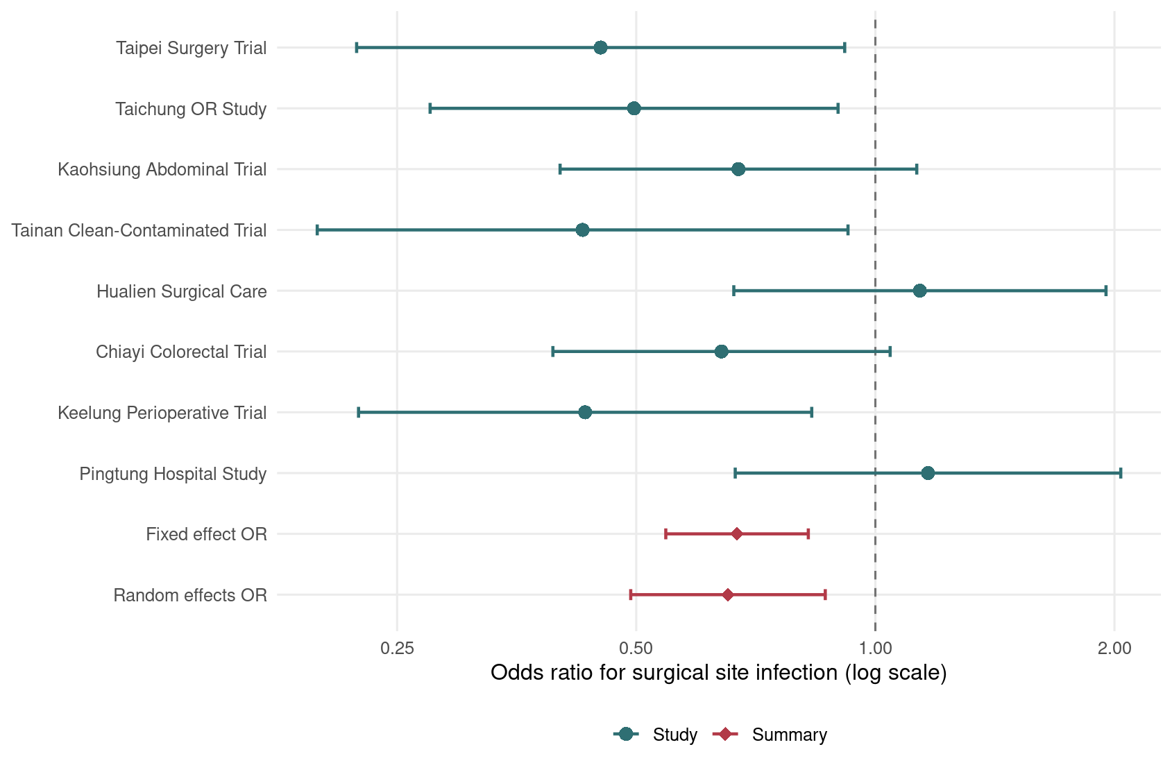
Figure 3.1: 圍手術期抗生素對手術部位感染的 OR 森林圖。
森林圖中,無效果線 (line of no effect) 是 OR = 1。多數研究點估計在 1 左側,表示抗生素組感染勝算較低。
Code
subgroup_summary <- ssi_es |>
  group_by(setting) |>
  summarise(
    k = n(),
    theta = exp(meta_iv(log_or, se_log_or)$random["theta"]),
    lower = exp(meta_iv(log_or, se_log_or)$random["lower"]),
    upper = exp(meta_iv(log_or, se_log_or)$random["upper"]),
    i2 = meta_iv(log_or, se_log_or)$i2,
    .groups = "drop"
  )

kable(
  subgroup_summary,
  col.names = c("手術傷口類型", "研究數", "隨機效應 OR",
                "95% CI 下限", "95% CI 上限", "I-squared (%)"),
  digits = 3
)
| Clean-contaminated |
4 |
0.455 |
0.325 |
0.637 |
0 |
| Colorectal |
2 |
0.655 |
0.459 |
0.935 |
0 |
| Contaminated |
2 |
1.151 |
0.781 |
1.696 |
0 |
Code
ggplot(subgroup_summary, aes(x = theta, y = setting)) +
  geom_vline(xintercept = 1, linetype = "dashed", color = "grey45") +
  geom_errorbar(
    aes(xmin = lower, xmax = upper),
    orientation = "y",
    width = 0.18,
    color = "#355C7D",
    linewidth = 0.9
  ) +
  geom_point(size = 3.5, color = "#C06C84") +
  scale_x_log10(breaks = c(0.25, 0.5, 1, 2)) +
  labs(
    x = "Random-effects odds ratio (log scale)",
    y = NULL
  ) +
  theme_minimal(base_size = 12) +
  theme(panel.grid.minor = element_blank())
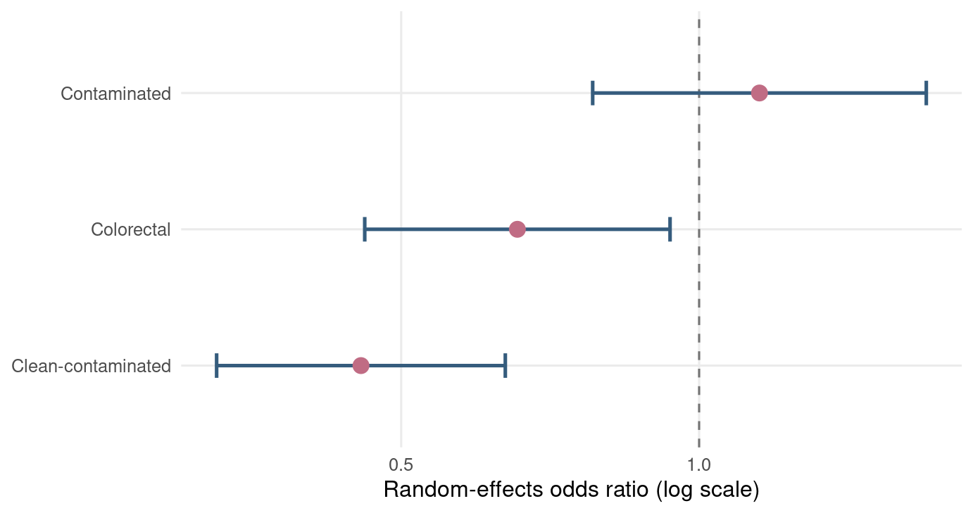
Figure 3.2: 依照手術傷口類型分層的隨機效應 OR 摘要。
次族群分析 (subgroup analysis) 可以幫助探索異質性來源,但要避免事後過度詮釋。若分組是看完資料才決定的,請把它當成假說生成,而不是結論生產線。
3.8 R 工作流程與套件提醒
本章完整 R 腳本儲存在 scripts/chapter3.R。你可以在專案根目錄執行:
Code
/usr/bin/Rscript scripts/chapter3.R
本章使用 dplyr、ggplot2、knitr 與 base R。正式分析時,建議同時使用 meta 或 metafor 檢查結果,例如 meta::metabin() 可直接執行 OR、RR、RD、Mantel–Haenszel、Peto 與隨機效應分析。目前本機已安裝 meta 與 metafor;若你的環境沒有,可執行:
Code
install.packages(c("meta", "metafor"))
套件很方便,但不要讓方便變成黑盒子。本章把公式展開,是為了讓你看到 OR、RR、RD 在資料表中如何長出來。
3.9 小結
本章介紹了二元結局統合分析的核心工具。OR、RR、RD 各有用途:OR 常見於模型與病例對照研究,RR 較容易臨床解讀,RD 最能表達絕對效益。當事件稀少或出現零事件時,分析方法的選擇會變得更敏感。
下一章會進一步處理異質性與 meta-regression。換句話說,我們不只問「平均效果是多少」,也要問「為什麼不同研究看起來不一樣」。這才是統合分析真正有趣,也真正需要小心的地方。
3.10 Glossary
| 二元結局 |
binary outcome |
| 手術部位感染 |
surgical site infection, SSI |
| 勝算 |
odds |
| 勝算比 |
odds ratio, OR |
| 風險比 |
risk ratio, RR |
| 風險差 |
risk difference, RD |
| 需治數 |
number needed to treat, NNT |
| Arcsine 差異 |
arcsine difference |
| 稀疏資料 |
sparse data |
| 零事件 |
zero event |
| 連續性校正 |
continuity correction |
| Peto 勝算比 |
Peto odds ratio |
| 觀察事件數減期望事件數 |
observed minus expected, O-E |
| 反變異數法 |
inverse-variance method |
| Mantel–Haenszel 方法 |
Mantel–Haenszel method |
| Peto 方法 |
Peto method |
| 固定效應模型 |
fixed-effect model |
| 隨機效應模型 |
random-effects model |
| 研究間變異 |
between-study variance |
| DerSimonian–Laird 方法 |
DerSimonian–Laird method |
| 異質性 |
heterogeneity |
| 無效果線 |
line of no effect |
| 次族群分析 |
subgroup analysis |