統合分析中的小研究效應 (Small-Study Effects in Meta-Analysis)

小研究效應、漏斗圖,以及那些沒有被看見的研究

5.1 本章學習目標

讀完本章後,你應該能夠:

  1. 說明小研究效應 (small-study effects) 與發表偏倚 (publication bias) 的差異。
  2. 使用漏斗圖 (funnel plot) 與 radial plot 檢視小研究效應。
  3. 執行 Begg 檢定、Egger 檢定與二元結局常用的 Peters 類檢定。
  4. 使用 trim-and-fill 方法調整可能的不對稱。
  5. 認識 Copas selection model 與 regression adjustment 的概念與限制。

統合分析最迷人的地方,是它試著把所有研究證據放到同一張桌上。但現實有點像期刊投稿界的晚餐邀約:結果顯著、效果很漂亮的小研究,往往比較容易被邀請入席;結果平淡的小研究,可能還在門口等候。這就是小研究效應與發表偏倚讓人頭痛的地方。

本章使用一個臨床情境:益生菌是否能預防兒童抗生素相關腹瀉。結局是是否發生腹瀉,效果量使用勝算比 (odds ratio, OR)。數值小於 1 代表益生菌可能有保護效果。

5.2 小研究效應是什麼?

小研究效應 (small-study effects) 指小型研究的效果估計系統性地不同於大型研究。它可能來自發表偏倚 (publication bias),也可能來自研究品質較差、選擇性報告、族群不同、介入執行較密集,或單純偶然。

發表偏倚只是小研究效應的一種可能原因。看到漏斗圖不對稱時,不要立刻說「一定是發表偏倚」。統計圖不喜歡被栽贓,它只是提醒我們:這裡有東西值得查。

Code
binary_effects <- function(dat) {
  dat |>
    mutate(
      a = event_tx,
      b = total_tx - event_tx,
      c = event_ctrl,
      d = total_ctrl - event_ctrl,
      n_total = total_tx + total_ctrl,
      log_or = log((a * d) / (b * c)),
      vi = 1 / a + 1 / b + 1 / c + 1 / d,
      se = sqrt(vi),
      or = exp(log_or),
      ci_low = exp(log_or - 1.96 * se),
      ci_high = exp(log_or + 1.96 * se)
    )
}
Code
diarrhea <- tibble::tibble(
  study = c("Taipei Pediatric Trial", "Taichung Ward Study",
            "Kaohsiung Multicenter Trial", "Tainan Outpatient Trial",
            "Hualien Community Trial", "Chiayi Clinic Study",
            "Keelung Probiotic Trial", "Pingtung Rural Study",
            "Miaoli Family Practice", "Yilan Hospital Trial",
            "Nantou Small Trial", "Taitung Pilot Study",
            "Large Asia-Pacific Trial", "Large Taiwan Network Trial"),
  event_tx = c(18, 16, 42, 13, 9, 11, 8, 6, 7, 21, 5, 4, 88, 74),
  total_tx = c(180, 150, 420, 120, 92, 110, 80, 70, 76, 210, 58, 52, 900, 780),
  event_ctrl = c(34, 30, 68, 29, 25, 26, 22, 18, 19, 39, 17, 14, 112, 98),
  total_ctrl = c(178, 148, 418, 118, 90, 108, 82, 72, 78, 208, 60, 54, 895, 775),
  risk_of_bias = c("Some concerns", "Some concerns", "Low", "Some concerns",
                   "High", "Some concerns", "High", "High", "High",
                   "Some concerns", "High", "High", "Low", "Low")
)

dia_es <- binary_effects(diarrhea)

kable(
  dia_es |>
    transmute(研究 = study, `總樣本數` = n_total, `偏差風險` = risk_of_bias,
              `OR` = or, `95% CI` = sprintf("%.2f to %.2f", ci_low, ci_high)),
  digits = 2
)
研究 總樣本數 偏差風險 OR 95% CI
Taipei Pediatric Trial 358 Some concerns 0.47 0.25 to 0.87
Taichung Ward Study 298 Some concerns 0.47 0.24 to 0.90
Kaohsiung Multicenter Trial 838 Low 0.57 0.38 to 0.86
Tainan Outpatient Trial 238 Some concerns 0.37 0.18 to 0.76
Hualien Community Trial 182 High 0.28 0.12 to 0.65
Chiayi Clinic Study 218 Some concerns 0.35 0.16 to 0.75
Keelung Probiotic Trial 162 High 0.30 0.13 to 0.73
Pingtung Rural Study 142 High 0.28 0.10 to 0.76
Miaoli Family Practice 154 High 0.32 0.12 to 0.80
Yilan Hospital Trial 418 Some concerns 0.48 0.27 to 0.85
Nantou Small Trial 118 High 0.24 0.08 to 0.70
Taitung Pilot Study 106 High 0.24 0.07 to 0.78
Large Asia-Pacific Trial 1795 Low 0.76 0.56 to 1.02
Large Taiwan Network Trial 1555 Low 0.72 0.53 to 1.00
Code
fit_fe <- rma.uni(yi = log_or, vi = vi, data = dia_es, method = "FE")
fit_re <- rma.uni(yi = log_or, vi = vi, data = dia_es, method = "DL")

kable(
  tibble::tibble(
    model = c("Fixed effect", "Random effects"),
    OR = exp(c(fit_fe$b[1], fit_re$b[1])),
    lower = exp(c(fit_fe$ci.lb, fit_re$ci.lb)),
    upper = exp(c(fit_fe$ci.ub, fit_re$ci.ub)),
    tau2 = c(0, fit_re$tau2),
    i2 = c(NA_real_, fit_re$I2)
  ),
  col.names = c("模型", "合併 OR", "95% CI 下限", "95% CI 上限", "tau-squared", "I-squared"),
  digits = 3
)
模型 合併 OR 95% CI 下限 95% CI 上限 tau-squared I-squared
Fixed effect 0.544 0.469 0.631 0.000 NA
Random effects 0.469 0.377 0.583 0.061 41.267

5.3 小研究效應的圖形檢視

5.3.1 漏斗圖

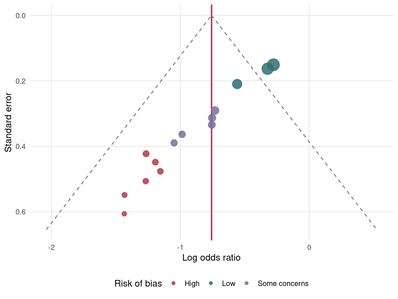
漏斗圖 (funnel plot) 把每個研究的效果估計放在 x 軸,精確度或標準誤放在 y 軸。大型研究標準誤小,通常在上方;小型研究標準誤大,會散在下方。若沒有小研究效應,點大致會以合併效果為中心呈現對稱漏斗。

Code
funnel_plot <- ggplot(dia_es, aes(x = log_or, y = se)) +
  geom_vline(xintercept = as.numeric(fit_re$b[1]), color = "#B23A48", linewidth = 0.9) +
  geom_line(
    data = tibble::tibble(
      se = seq(0, max(dia_es$se) * 1.08, length.out = 100),
      left = as.numeric(fit_re$b[1]) - 1.96 * se,
      right = as.numeric(fit_re$b[1]) + 1.96 * se
    ),
    aes(x = left, y = se),
    inherit.aes = FALSE,
    linetype = "dashed",
    color = "grey45"
  ) +
  geom_line(
    data = tibble::tibble(
      se = seq(0, max(dia_es$se) * 1.08, length.out = 100),
      left = as.numeric(fit_re$b[1]) - 1.96 * se,
      right = as.numeric(fit_re$b[1]) + 1.96 * se
    ),
    aes(x = right, y = se),
    inherit.aes = FALSE,
    linetype = "dashed",
    color = "grey45"
  ) +
  geom_point(aes(size = n_total, color = risk_of_bias), alpha = 0.85) +
  scale_y_reverse() +
  scale_size_continuous(range = c(2.5, 7), guide = "none") +
  scale_color_manual(values = c("Low" = "#2F6F73", "Some concerns" = "#7A6F9B", "High" = "#B23A48")) +
  labs(x = "Log odds ratio", y = "Standard error", color = "Risk of bias") +
  theme_minimal(base_size = 12) +
  theme(legend.position = "bottom", panel.grid.minor = element_blank())

funnel_plot

Figure 5.1: 益生菌預防兒童抗生素相關腹瀉研究的漏斗圖。

這張圖中,小型研究較常出現在較強保護效果的一側,而大型研究較接近中間。這種不對稱可能是小研究效應,但原因仍需搭配研究品質、登錄資料、灰色文獻與敏感度分析判斷。

5.3.2 Radial plot

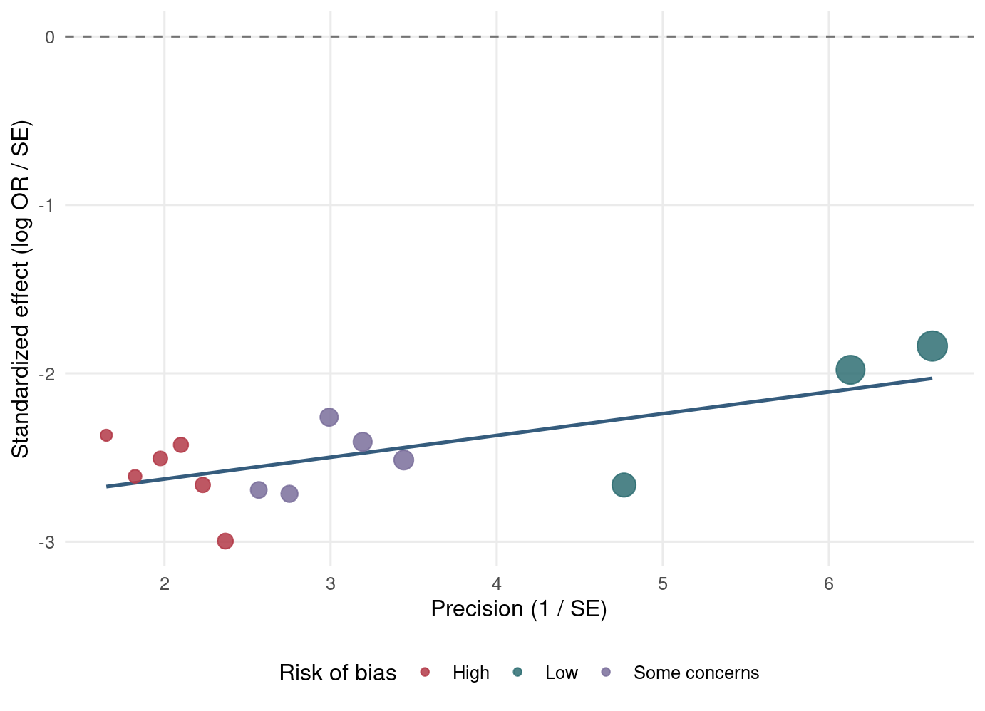
Radial plot 又稱 Galbraith plot,常把標準化效果放在 y 軸、精確度放在 x 軸。它有助於辨識離群研究,以及效果是否隨精確度改變。

Code
radial_data <- dia_es |>
  mutate(
    precision = 1 / se,
    standardized_effect = log_or / se
  )

ggplot(radial_data, aes(x = precision, y = standardized_effect)) +
  geom_hline(yintercept = 0, linetype = "dashed", color = "grey45") +
  geom_smooth(method = "lm", se = FALSE, color = "#355C7D", linewidth = 0.9) +
  geom_point(aes(size = n_total, color = risk_of_bias), alpha = 0.85) +
  scale_size_continuous(range = c(2.5, 7), guide = "none") +
  scale_color_manual(values = c("Low" = "#2F6F73", "Some concerns" = "#7A6F9B", "High" = "#B23A48")) +
  labs(x = "Precision (1 / SE)", y = "Standardized effect (log OR / SE)", color = "Risk of bias") +
  theme_minimal(base_size = 12) +
  theme(legend.position = "bottom", panel.grid.minor = element_blank())

Figure 5.2: Radial plot 用來檢視標準化效果與研究精確度的關係。

5.4 小研究效應的統計檢定

5.4.1 Begg 與 Egger 的古典檢定

Begg 檢定 (Begg test) 使用秩相關概念檢視效果量與其變異是否相關。Egger 檢定 (Egger test) 則使用迴歸方法檢查 funnel plot asymmetry。兩者都需要謹慎解讀,尤其研究數少於 10 時,檢定力通常不足;研究間異質性高時,也可能誤導。

Code
egger <- regtest(fit_re, model = "lm", predictor = "sei")
begg <- ranktest(fit_re)

test_tbl <- tibble::tibble(
  test = c("Egger regression", "Begg rank correlation"),
  statistic = c(unname(egger$zval), unname(begg$tau)),
  p_value = c(egger$pval, begg$pval)
)

kable(test_tbl, col.names = c("檢定", "統計量", "p 值"), digits = 3)
檢定 統計量 p 值
Egger regression -19.934 0
Begg rank correlation -0.802 0

檢定顯著不等於「一定有發表偏倚」,不顯著也不等於「一定沒問題」。它比較像煙霧警報器:響了要查,但沒響不代表整棟樓永遠安全。

5.4.2 二元結局的修正版檢定

二元結局 (binary outcome) 的 OR 與標準誤常有數學相關,這會影響 Egger 檢定。Peters test 是常用修正版之一,概念上以總樣本數的倒數作為小研究程度指標。以下示範 Peters 類加權迴歸:

Code
peters_fit <- lm(log_or ~ I(1 / n_total), weights = 1 / vi, data = dia_es)
peters_coef <- coef(summary(peters_fit))

kable(
  tibble::tibble(
    term = rownames(peters_coef),
    estimate = peters_coef[, "Estimate"],
    se = peters_coef[, "Std. Error"],
    statistic = peters_coef[, "t value"],
    p_value = peters_coef[, "Pr(>|t|)"]
  ),
  col.names = c("項目", "係數", "SE", "統計量", "p 值"),
  digits = 3
)
項目 係數 SE 統計量 p 值
(Intercept) -0.264 0.035 -7.496 0
I(1/n_total) -152.094 10.952 -13.887 0

二元結局的小研究效應檢定還包括 Harbord test 與 Rücker 類方法。實務上,不建議只靠單一檢定做結論;應搭配圖形、敏感度分析與研究品質評估。

5.5 小研究效應的調整方法

5.5.1 Trim-and-fill 方法

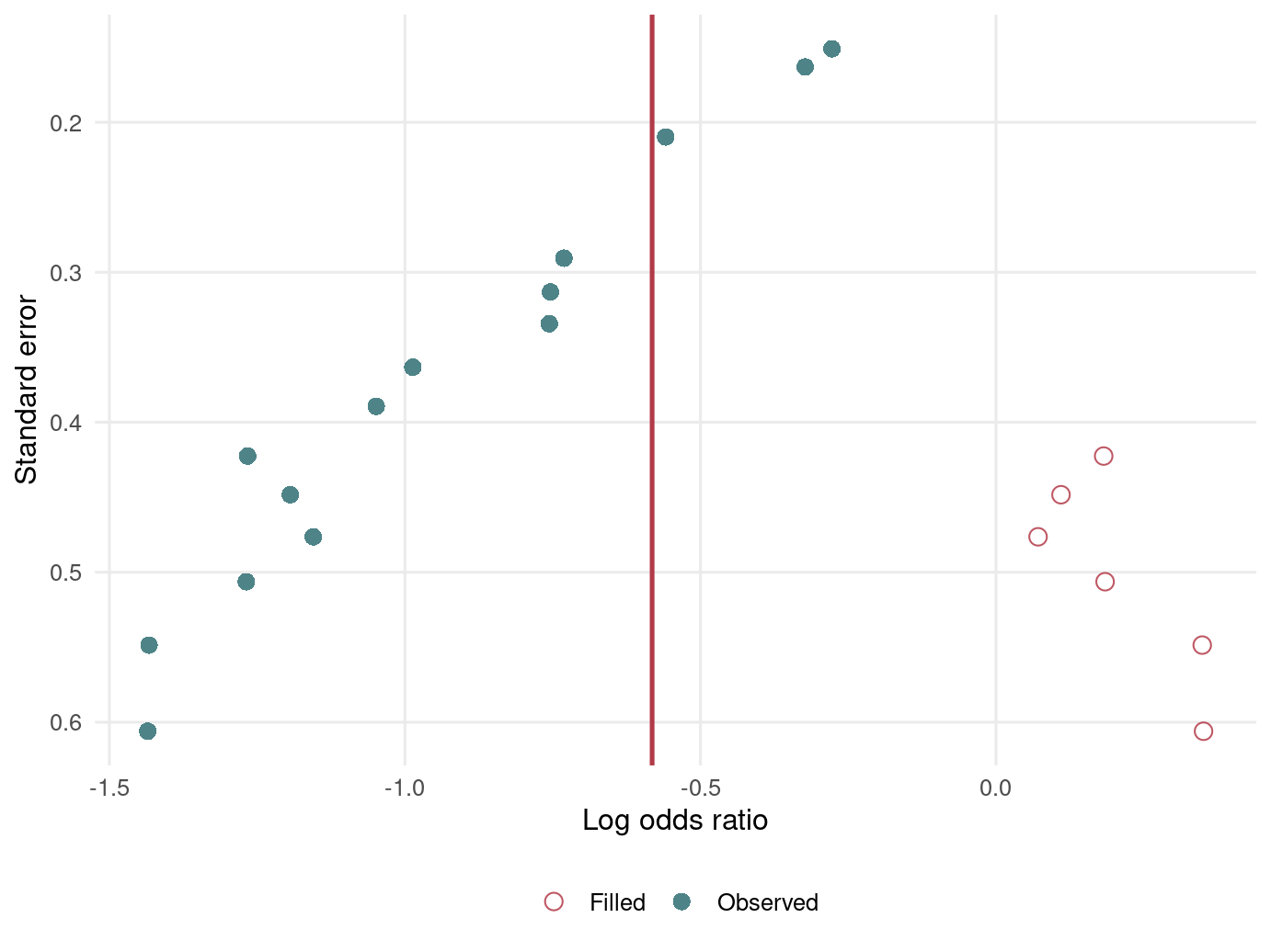
Trim-and-fill 方法 (trim-and-fill method) 會先修剪造成不對稱的研究,再填補推測缺少的研究,最後重新估計合併效果。它很有教學直覺,但不是失蹤研究偵測器;若不對稱來自異質性或研究品質差異,trim-and-fill 可能會過度簡化問題。

Code
tf <- trimfill(fit_re)

tf_tbl <- tibble::tibble(
  item = c("Observed random-effects OR", "Trim-and-fill OR", "Number of filled studies"),
  value = c(exp(fit_re$b[1]), exp(tf$b[1]), sum(tf$fill))
)

kable(tf_tbl, col.names = c("項目", "數值"), digits = 3)
項目 數值
Observed random-effects OR 0.469
Trim-and-fill OR 0.559
Number of filled studies 6.000
Code
tf_data <- tibble::tibble(
  log_or = c(dia_es$log_or, tf$yi.f[tf$fill]),
  se = sqrt(c(dia_es$vi, tf$vi.f[tf$fill])),
  type = c(rep("Observed", nrow(dia_es)), rep("Filled", sum(tf$fill)))
)

ggplot(tf_data, aes(x = log_or, y = se)) +
  geom_vline(xintercept = as.numeric(tf$b[1]), color = "#B23A48", linewidth = 0.9) +
  geom_point(aes(shape = type, color = type), size = 3, alpha = 0.85) +
  scale_y_reverse() +
  scale_color_manual(values = c("Observed" = "#2F6F73", "Filled" = "#B23A48")) +
  scale_shape_manual(values = c("Observed" = 16, "Filled" = 1)) +
  labs(x = "Log odds ratio", y = "Standard error", color = NULL, shape = NULL) +
  theme_minimal(base_size = 12) +
  theme(legend.position = "bottom", panel.grid.minor = element_blank())

Figure 5.3: Trim-and-fill 方法填補推測缺少研究後的漏斗圖。

5.5.2 Copas selection model

Copas selection model 是選擇模型 (selection model) 的一種,直接建模「研究被觀察到」的機率與研究精確度、結果大小之間的關係。它比 trim-and-fill 更明確地處理選擇機制,但需要更多假設,因此常作為敏感度分析,而不是唯一答案。

Code
meta_obj <- metagen(
  TE = log_or,
  seTE = se,
  studlab = study,
  data = dia_es,
  sm = "OR",
  common = FALSE,
  random = TRUE,
  method.tau = "DL",
  backtransf = TRUE
)

copas_fit <- copas(meta_obj, silent = TRUE)

copas_sensitivity <- tibble::tibble(
  selection_scenario = seq_along(copas_fit$TE.slope),
  estimated_unpublished = copas_fit$N.unpubl,
  log_or = copas_fit$TE.slope,
  lower = copas_fit$lower.slope,
  upper = copas_fit$upper.slope,
  or = exp(log_or),
  or_low = exp(lower),
  or_high = exp(upper)
)

kable(
  copas_sensitivity |>
    transmute(
      `選擇情境` = selection_scenario,
      `估計未發表研究數` = estimated_unpublished,
      `OR` = or,
      `95% CI` = sprintf("%.2f to %.2f", or_low, or_high)
    ),
  col.names = c("選擇情境", "估計未發表研究數", "OR", "95% CI"),
  digits = 3
)
選擇情境 估計未發表研究數 OR 95% CI
1 0.000 0.468 0.36 to 0.60
2 0.178 0.472 0.37 to 0.61
3 1.418 0.496 0.38 to 0.64
4 2.864 0.522 0.40 to 0.67
5 4.379 0.547 0.42 to 0.70
6 5.148 0.599 0.46 to 0.77
7 7.074 0.616 0.48 to 0.80
8 10.371 0.640 0.50 to 0.83
9 14.640 0.665 0.52 to 0.86

Copas 模型的重點不是給出「真正答案」,而是檢查結論對不同選擇機制是否敏感。若調整後效果大幅改變,報告時就應更保守;若結論相對穩定,也仍要說明模型假設。

5.5.3 Regression adjustment

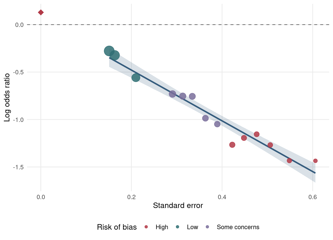
Regression adjustment 以研究精確度或標準誤作為解釋變項,估計當標準誤趨近於 0 時的效果,也就是理想大型研究的效果。這常被稱為 limit meta-analysis 的想法。

Code
fit_reg_adj <- rma.uni(yi = log_or, vi = vi, mods = ~ se, data = dia_es, method = "DL")
limit_est <- predict(fit_reg_adj, newmods = 0)

summary_tbl <- tibble::tibble(
  method = c("Fixed effect", "Random effects", "Trim-and-fill",
             "Regression adjustment at SE = 0"),
  log_or = c(as.numeric(fit_fe$b[1]), as.numeric(fit_re$b[1]),
             as.numeric(tf$b[1]), limit_est$pred),
  lower = c(fit_fe$ci.lb, fit_re$ci.lb, tf$ci.lb, limit_est$ci.lb),
  upper = c(fit_fe$ci.ub, fit_re$ci.ub, tf$ci.ub, limit_est$ci.ub)
) |>
  mutate(or = exp(log_or), or_low = exp(lower), or_high = exp(upper))

kable(
  summary_tbl |>
    transmute(方法 = method, `OR` = or, `95% CI` = sprintf("%.2f to %.2f", or_low, or_high)),
  digits = 3
)
方法 OR 95% CI
Fixed effect 0.544 0.47 to 0.63
Random effects 0.469 0.38 to 0.58
Trim-and-fill 0.559 0.45 to 0.69
Regression adjustment at SE = 0 1.138 0.81 to 1.61
Code
ggplot(dia_es, aes(x = se, y = log_or)) +
  geom_hline(yintercept = 0, linetype = "dashed", color = "grey45") +
  geom_smooth(method = "lm", se = TRUE, color = "#355C7D", fill = "#355C7D", alpha = 0.18) +
  geom_point(aes(size = 1 / vi, color = risk_of_bias), alpha = 0.85) +
  geom_point(data = tibble::tibble(se = 0, log_or = limit_est$pred),
             aes(x = se, y = log_or), inherit.aes = FALSE,
             color = "#B23A48", size = 4, shape = 18) +
  scale_size_continuous(range = c(2.5, 7), guide = "none") +
  scale_color_manual(values = c("Low" = "#2F6F73", "Some concerns" = "#7A6F9B", "High" = "#B23A48")) +
  labs(x = "Standard error", y = "Log odds ratio", color = "Risk of bias") +
  theme_minimal(base_size = 12) +
  theme(legend.position = "bottom", panel.grid.minor = element_blank())

Figure 5.4: 以標準誤為解釋變項的 regression adjustment。紅色菱形為 SE = 0 的推估效果。

5.6 R 工作流程與套件提醒

本章完整 R 腳本儲存在 scripts/chapter5.R。你可以在專案根目錄執行:

Code
/usr/bin/Rscript scripts/chapter5.R

本章可完整執行所需套件為 metaformetametasensggplot2dplyrknitr,目前本機皆已安裝。若你的環境尚未安裝,可執行:

Code
install.packages(c("metafor", "meta", "metasens"))

5.7 小結

小研究效應是統合分析中最需要謙虛的主題之一。漏斗圖、Begg/Egger/Peters 檢定、trim-and-fill 與 regression adjustment 都能提供線索,但沒有任何一個方法能單獨證明發表偏倚。好的報告應該把圖形、統計檢定、研究品質、登錄紀錄與灰色文獻搜尋放在一起解讀。

下一章會討論遺漏資料。那會是另一種「看不到」:不是研究沒被發表,而是病人、結果或精確度沒有完整出現在資料表裡。統計人生就是這樣,最難的常常不是已知的數字,而是沉默的空格。

5.8 Glossary

中文 English
小研究效應 small-study effects
發表偏倚 publication bias
漏斗圖 funnel plot
Radial plot radial plot
Galbraith plot Galbraith plot
勝算比 odds ratio, OR
標準誤 standard error, SE
偏差風險 risk of bias
漏斗圖不對稱 funnel plot asymmetry
Begg 檢定 Begg test
Egger 檢定 Egger test
Peters test Peters test
Harbord test Harbord test
Trim-and-fill 方法 trim-and-fill method
Copas selection model Copas selection model
選擇模型 selection model
敏感度分析 sensitivity analysis
Regression adjustment regression adjustment
Limit meta-analysis limit meta-analysis
灰色文獻 grey literature