異質性與統合迴歸 (Heterogeneity and Meta-Regression)

當研究不一樣時,不要急著責怪資料

4.1 本章學習目標

讀完本章後,你應該能夠:

  1. 說明異質性 (heterogeneity) 的臨床、方法學與統計來源。
  2. 解讀 \(Q\)\(I^2\)\(H^2\)\(\tau^2\)\(\tau\) 等異質性指標。
  3. 執行次族群差異檢定 (test for subgroup differences),並比較固定效應、分組各自 \(\tau^2\)、共同 \(\tau^2\) 的想法。
  4. 使用 meta-regression 探索類別共變項 (categorical covariate) 與連續共變項 (continuous covariate)。
  5. 分辨「探索異質性」與「替資料編故事」之間那條細細但很重要的線。

前面幾章我們已經知道,統合分析不是把研究結果丟進果汁機。到了本章,我們要正面處理一件現實:研究常常不一樣。族群不同、介入強度不同、追蹤時間不同、基準風險不同,結果自然可能不同。異質性不是壞學生,它常常是在提醒我們:「臨床脈絡還沒講完。」

本章使用的臨床範例是遠距心理照護介入是否能改善憂鬱症狀。結局是 PHQ-9 分數變化的平均差 (mean difference, MD);數值越負,代表介入組症狀改善較多。

4.2 異質性的來源

異質性 (heterogeneity) 可粗略分成三類:

  • 臨床異質性 (clinical heterogeneity):病人年齡、疾病嚴重度、共病、基準風險、照護場域不同。
  • 方法學異質性 (methodological heterogeneity):隨機分派、盲法、失訪處理、結局測量時間、偏差風險不同。
  • 統計異質性 (statistical heterogeneity):研究效果量之間的差異超過抽樣誤差可解釋的程度。

臨床與方法學異質性是原因,統計異質性是數字上看到的結果。看到高 \(I^2\) 時,不要只說「異質性很高」就下台一鞠躬;真正重要的是回去問:這些研究到底哪裡不一樣?

Code
telehealth <- tibble::tibble(
  study = c("Taipei Mood Trial", "Taichung Primary Care Study",
            "Kaohsiung Digital CBT", "Tainan Collaborative Care",
            "Hualien Rural Telehealth", "Chiayi App-Guided Trial",
            "Keelung Nurse Coaching", "Pingtung Community Study",
            "Miaoli Older Adult Trial", "Yilan Brief CBT Study",
            "Nantou Stepped Care", "Taitung Indigenous Health Trial"),
  population = c("Adult", "Adult", "Adult", "Adult", "Rural", "Adult",
                 "Older adult", "Rural", "Older adult", "Adult",
                 "Older adult", "Rural"),
  sessions = c(8, 6, 10, 7, 4, 5, 6, 3, 5, 4, 7, 4),
  n_tx = c(120, 95, 140, 110, 78, 130, 86, 72, 90, 88, 94, 70),
  mean_tx = c(-8.5, -6.2, -10.4, -7.4, -3.8, -5.8, -4.6, -2.9, -4.1, -4.9, -5.2, -3.1),
  sd_tx = c(8.8, 7.9, 9.1, 8.0, 7.5, 8.2, 7.7, 7.1, 7.9, 7.6, 8.0, 7.3),
  n_ctrl = c(118, 98, 136, 108, 80, 128, 84, 74, 88, 90, 92, 72),
  mean_ctrl = c(-4.1, -3.2, -4.5, -3.9, -2.4, -3.0, -2.8, -2.0, -2.2, -2.9, -2.6, -1.9),
  sd_ctrl = c(8.5, 8.1, 8.9, 8.2, 7.2, 8.0, 7.5, 7.0, 7.6, 7.5, 7.8, 7.1)
)

tele_es <- telehealth |>
  mutate(
    md = mean_tx - mean_ctrl,
    vi = sd_tx^2 / n_tx + sd_ctrl^2 / n_ctrl,
    se = sqrt(vi),
    ci_low = md - 1.96 * se,
    ci_high = md + 1.96 * se,
    population = factor(population, levels = c("Adult", "Older adult", "Rural"))
  )

kable(
  tele_es |>
    transmute(研究 = study, 族群 = population, 療程數 = sessions,
              `MD` = md, `SE` = se, `95% CI` = sprintf("%.2f to %.2f", ci_low, ci_high)),
  digits = 2
)
研究 族群 療程數 MD SE 95% CI
Taipei Mood Trial Adult 8 -4.4 1.12 -6.60 to -2.20
Taichung Primary Care Study Adult 6 -3.0 1.15 -5.26 to -0.74
Kaohsiung Digital CBT Adult 10 -5.9 1.08 -8.02 to -3.78
Tainan Collaborative Care Adult 7 -3.5 1.10 -5.65 to -1.35
Hualien Rural Telehealth Rural 4 -1.4 1.17 -3.69 to 0.89
Chiayi App-Guided Trial Adult 5 -2.8 1.01 -4.78 to -0.82
Keelung Nurse Coaching Older adult 6 -1.8 1.17 -4.08 to 0.48
Pingtung Community Study Rural 3 -0.9 1.17 -3.19 to 1.39
Miaoli Older Adult Trial Older adult 5 -1.9 1.16 -4.18 to 0.38
Yilan Brief CBT Study Adult 4 -2.0 1.13 -4.22 to 0.22
Nantou Stepped Care Older adult 7 -2.6 1.16 -4.87 to -0.33
Taitung Indigenous Health Trial Rural 4 -1.2 1.21 -3.57 to 1.17

4.3 異質性的量測

常見異質性指標包括 Cochran’s \(Q\)\(I^2\)\(H^2\)\(\tau^2\)\(\tau\)。本章用 metafor 套件進行分析。metafor::rma.uni() 是統合分析與 meta-regression 很常用的函數。

Code
fit_fe <- rma.uni(yi = md, vi = vi, data = tele_es, method = "FE")
fit_re <- rma.uni(yi = md, vi = vi, data = tele_es, method = "DL")

summary_tbl <- tibble::tibble(
  model = c("Fixed effect", "Random effects"),
  estimate = c(as.numeric(fit_fe$b[1]), as.numeric(fit_re$b[1])),
  lower = c(fit_fe$ci.lb, fit_re$ci.lb),
  upper = c(fit_fe$ci.ub, fit_re$ci.ub),
  tau2 = c(0, fit_re$tau2),
  i2 = c(NA_real_, fit_re$I2)
)

heterogeneity_tbl <- tibble::tibble(
  quantity = c("Q", "df", "Q test p-value", "tau-squared", "tau", "I-squared (%)", "H-squared"),
  value = c(fit_re$QE, fit_re$k - 1, fit_re$QEp, fit_re$tau2,
            sqrt(fit_re$tau2), fit_re$I2, fit_re$H2)
)

kable(summary_tbl, col.names = c("模型", "合併 MD", "95% CI 下限", "95% CI 上限", "tau-squared", "I-squared"), digits = 2)
模型 合併 MD 95% CI 下限 95% CI 上限 tau-squared I-squared
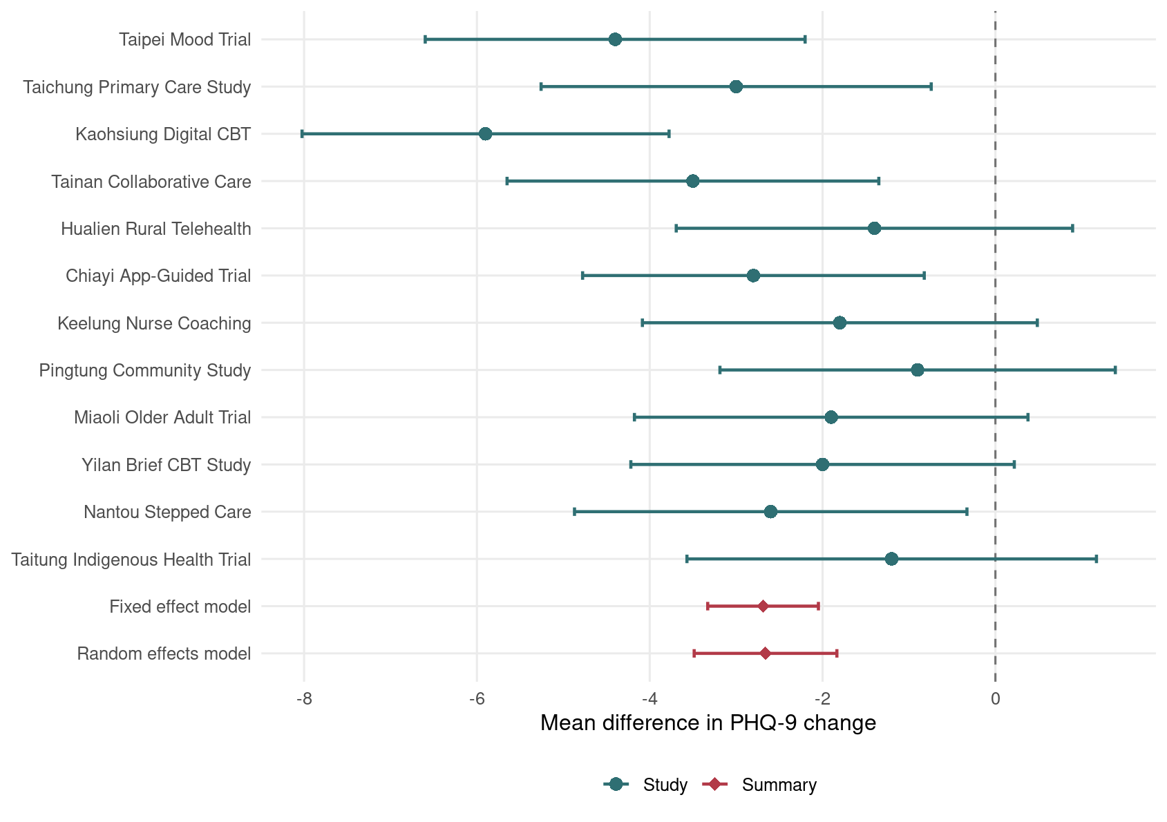
Fixed effect -2.69 -3.33 -2.05 0.00 NA
Random effects -2.66 -3.49 -1.83 0.84 39.7
Code
kable(heterogeneity_tbl, col.names = c("統計量", "數值"), digits = 3)
統計量 數值
Q 18.241
df 11.000
Q test p-value 0.076
tau-squared 0.844
tau 0.919
I-squared (%) 39.696
H-squared 1.658

\(Q\) 檢定 (Q test) 的虛無假設是所有研究共享同一真實效果。\(I^2\) 描述總變異中有多少比例可歸因於異質性。\(\tau^2\) 是研究間變異 (between-study variance),\(\tau\) 則回到原效果量尺度,因此在 MD 的例子中比較容易臨床解讀。

Code
forest_data <- bind_rows(
  tele_es |>
    transmute(study, estimate = md, lower = ci_low, upper = ci_high, type = "Study"),
  tibble::tibble(
    study = c("Fixed effect model", "Random effects model"),
    estimate = c(as.numeric(fit_fe$b[1]), as.numeric(fit_re$b[1])),
    lower = c(fit_fe$ci.lb, fit_re$ci.lb),
    upper = c(fit_fe$ci.ub, fit_re$ci.ub),
    type = "Summary"
  )
) |>
  mutate(study = factor(study, levels = rev(study)))

ggplot(forest_data, aes(x = estimate, y = study)) +
  geom_vline(xintercept = 0, linetype = "dashed", color = "grey45") +
  geom_errorbar(aes(xmin = lower, xmax = upper, color = type),
                orientation = "y", width = 0.18, linewidth = 0.8) +
  geom_point(aes(color = type, shape = type), size = 3.1) +
  scale_color_manual(values = c("Study" = "#2F6F73", "Summary" = "#B23A48")) +
  scale_shape_manual(values = c("Study" = 16, "Summary" = 18)) +
  labs(x = "Mean difference in PHQ-9 change", y = NULL, color = NULL, shape = NULL) +
  theme_minimal(base_size = 12) +
  theme(legend.position = "bottom", panel.grid.minor = element_blank())

Figure 4.1: 遠距心理照護介入對 PHQ-9 變化的森林圖,顯示固定效應與隨機效應合併估計。

4.4 次族群差異檢定

次族群分析 (subgroup analysis) 可用來探索異質性來源。本例依族群分成成人、年長者與偏鄉族群。請注意,次族群分析最好事先規劃;事後看圖說故事,很容易把統計課變成占星術課。

4.4.1 固定效應模型

固定效應次族群檢定把研究間差異視為抽樣誤差,並檢定不同 subgroup 的合併效果是否相同。

Code
fit_cat_fe <- rma.uni(yi = md, vi = vi, mods = ~ population, data = tele_es, method = "FE")

kable(
  tibble::tibble(
    test = "Fixed effect subgroup test",
    QM = fit_cat_fe$QM,
    df = fit_cat_fe$m,
    p_value = fit_cat_fe$QMp
  ),
  col.names = c("檢定", "QM", "df", "p 值"),
  digits = 3
)
檢定 QM df p 值
Fixed effect subgroup test 9.944 2 0.007

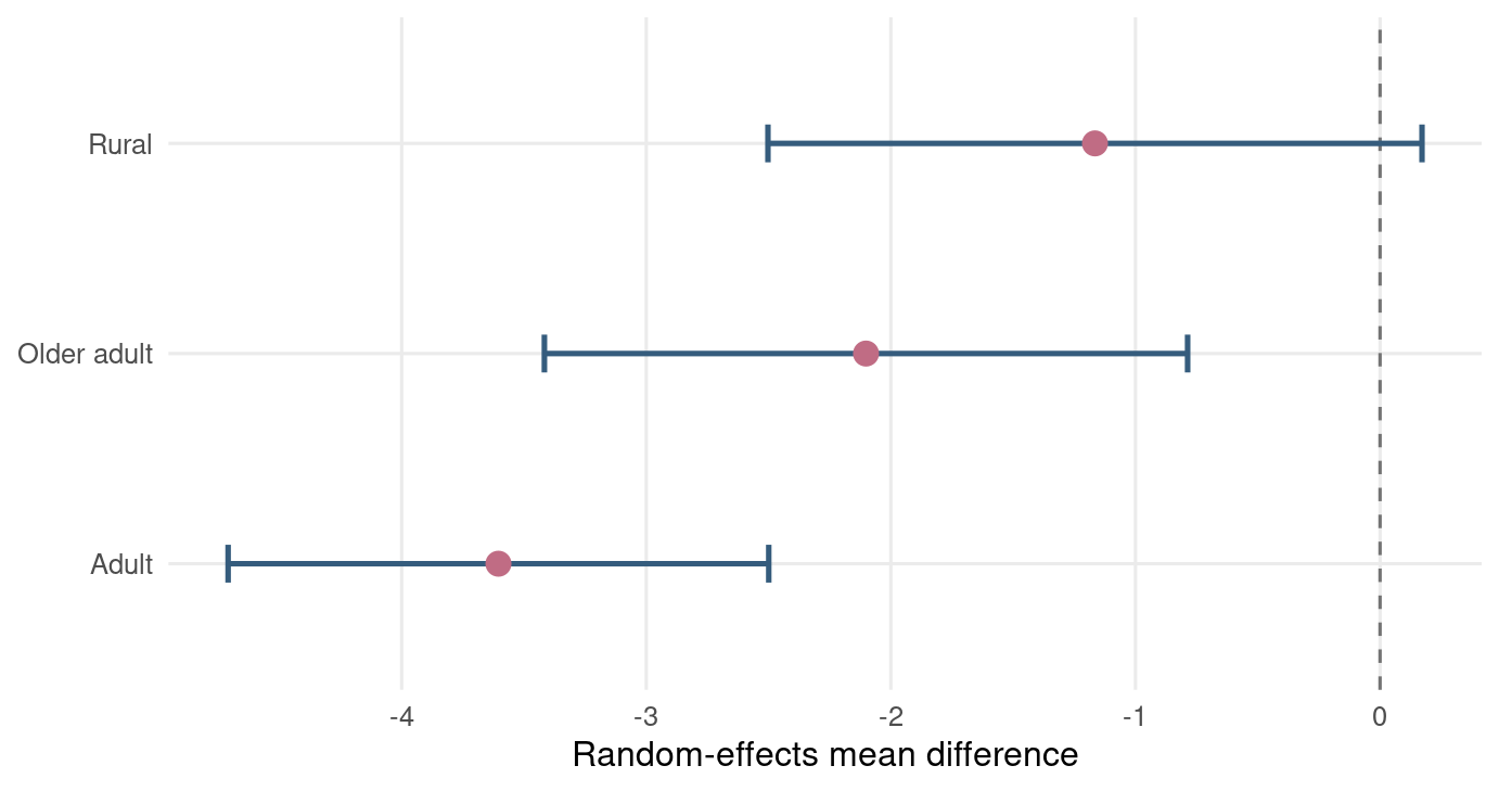
4.4.2 分組各自估計 \(\tau^2\) 的隨機效應模型

如果我們認為各次族群內部的異質性可能不同,可以讓每個 subgroup 各自估計 \(\tau^2\)。這比較彈性,但每組研究數少時,\(\tau^2\) 會估得不穩。

Code
separate_tau <- tele_es |>
  group_by(population) |>
  group_modify(\(.x, .y) {
    fit <- rma.uni(yi = md, vi = vi, data = .x, method = "DL")
    tibble::tibble(
      k = fit$k,
      estimate = as.numeric(fit$b[1]),
      lower = fit$ci.lb,
      upper = fit$ci.ub,
      tau2 = fit$tau2,
      i2 = fit$I2
    )
  }) |>
  ungroup()

kable(separate_tau, col.names = c("族群", "研究數", "合併 MD", "95% CI 下限", "95% CI 上限", "tau-squared", "I-squared"), digits = 2)
族群 研究數 合併 MD 95% CI 下限 95% CI 上限 tau-squared I-squared
Adult 6 -3.60 -4.71 -2.50 0.7 36.88
Older adult 3 -2.10 -3.42 -0.79 0.0 0.00
Rural 3 -1.17 -2.50 0.17 0.0 0.00
Code
ggplot(separate_tau, aes(x = estimate, y = population)) +
  geom_vline(xintercept = 0, linetype = "dashed", color = "grey45") +
  geom_errorbar(aes(xmin = lower, xmax = upper), orientation = "y",
                width = 0.18, color = "#355C7D", linewidth = 0.9) +
  geom_point(size = 3.5, color = "#C06C84") +
  labs(x = "Random-effects mean difference", y = NULL) +
  theme_minimal(base_size = 12) +
  theme(panel.grid.minor = element_blank())

Figure 4.2: 各族群使用各自 \(\tau^2\) 的隨機效應摘要。

4.4.3 共同 \(\tau^2\) 的隨機效應模型

若我們認為各 subgroup 的研究間變異可共享同一個 \(\tau^2\),可以使用共同 \(\tau^2\) 的隨機效應 meta-regression。這在研究數有限時常較穩定。

Code
fit_cat_common <- rma.uni(yi = md, vi = vi, mods = ~ population, data = tele_es, method = "DL")

cat_tbl <- tibble::tibble(
  model = c("Fixed effect subgroup test", "Random effects common tau"),
  qm = c(fit_cat_fe$QM, fit_cat_common$QM),
  df = c(fit_cat_fe$m, fit_cat_common$m),
  p_value = c(fit_cat_fe$QMp, fit_cat_common$QMp),
  tau2 = c(0, fit_cat_common$tau2)
)

kable(cat_tbl, col.names = c("模型", "QM", "df", "p 值", "tau-squared"), digits = 3)
模型 QM df p 值 tau-squared
Fixed effect subgroup test 9.944 2 0.007 0
Random effects common tau 9.944 2 0.007 0

4.5 Meta-regression

Meta-regression 是把研究層級共變項加入統合分析模型,用來探索效果量是否隨研究特徵而改變。請記得:meta-regression 的單位是研究,不是個別病人。因此它很容易受到生態謬誤 (ecological fallacy) 影響。研究層級關聯不等於個人層級因果關係。

4.5.1 類別共變項

族群類型就是類別共變項 (categorical covariate)。前一節的 subgroup model 其實就是類別共變項的 meta-regression。

Code
kable(
  tibble::tibble(
    term = rownames(coef(summary(fit_cat_common))),
    estimate = coef(summary(fit_cat_common))[, "estimate"],
    se = coef(summary(fit_cat_common))[, "se"],
    z = coef(summary(fit_cat_common))[, "zval"],
    p_value = coef(summary(fit_cat_common))[, "pval"]
  ),
  col.names = c("項目", "係數", "SE", "z", "p 值"),
  digits = 3
)
項目 係數 SE z p 值
intrcpt -3.605 0.447 -8.057 0.000
populationOlder adult 1.503 0.806 1.864 0.062
populationRural 2.439 0.816 2.990 0.003

4.5.2 連續共變項

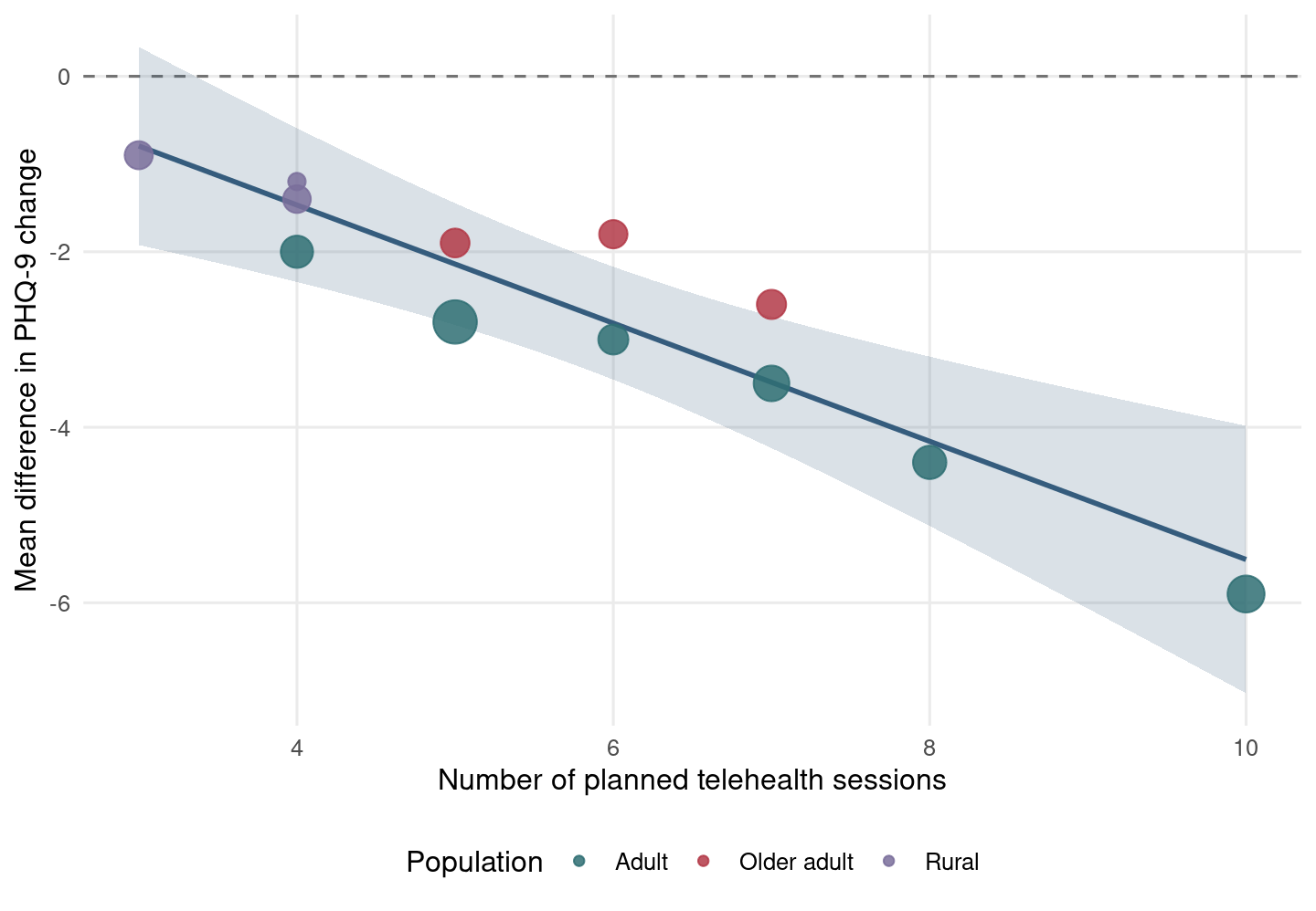
連續共變項 (continuous covariate) 的例子是遠距照護療程數。若療程數越多,介入效果是否越大?我們可以用 sessions 作為解釋變項。

Code
fit_sessions <- rma.uni(yi = md, vi = vi, mods = ~ sessions, data = tele_es, method = "DL")

metareg_tbl <- tibble::tibble(
  term = rownames(coef(summary(fit_sessions))),
  estimate = coef(summary(fit_sessions))[, "estimate"],
  se = coef(summary(fit_sessions))[, "se"],
  z = coef(summary(fit_sessions))[, "zval"],
  p_value = coef(summary(fit_sessions))[, "pval"]
)

kable(metareg_tbl, col.names = c("項目", "係數", "SE", "z", "p 值"), digits = 3)
項目 係數 SE z p 值
intrcpt 1.226 1.033 1.186 0.236
sessions -0.673 0.169 -3.993 0.000

斜率若為負,代表療程數越多,PHQ-9 改善越多。這很合理,但還不能直接說「多上一堂就一定多改善多少分」。療程數可能與治療品質、病人選擇、場域資源一起變動,統計模型只能幫我們照亮一部分房間。

Code
pred_grid <- tibble::tibble(sessions = seq(min(tele_es$sessions), max(tele_es$sessions), length.out = 100))
pred_obj <- predict(fit_sessions, newmods = pred_grid$sessions)
pred_grid <- pred_grid |>
  mutate(pred = pred_obj$pred, ci_low = pred_obj$ci.lb, ci_high = pred_obj$ci.ub)

ggplot(tele_es, aes(x = sessions, y = md)) +
  geom_hline(yintercept = 0, linetype = "dashed", color = "grey45") +
  geom_ribbon(data = pred_grid, aes(x = sessions, y = pred, ymin = ci_low, ymax = ci_high),
              inherit.aes = FALSE, alpha = 0.18, fill = "#355C7D") +
  geom_line(data = pred_grid, aes(x = sessions, y = pred), inherit.aes = FALSE,
            color = "#355C7D", linewidth = 1) +
  geom_point(aes(size = 1 / vi, color = population), alpha = 0.85) +
  scale_size_continuous(range = c(3, 8), guide = "none") +
  scale_color_manual(values = c("Adult" = "#2F6F73", "Older adult" = "#B23A48", "Rural" = "#7A6F9B")) +
  labs(x = "Number of planned telehealth sessions",
       y = "Mean difference in PHQ-9 change",
       color = "Population") +
  theme_minimal(base_size = 12) +
  theme(legend.position = "bottom", panel.grid.minor = element_blank())

Figure 4.3: 以療程數作為連續共變項的 meta-regression bubble plot。點的大小代表研究權重。

4.6 R 工作流程與套件提醒

本章完整 R 腳本儲存在 scripts/chapter4.R。你可以在專案根目錄執行:

Code
/usr/bin/Rscript scripts/chapter4.R

本章使用 metafor 進行 meta-regression。目前本機已安裝 metaformeta;若你的環境尚未安裝,可執行:

Code
install.packages(c("metafor", "meta"))

4.7 小結

本章的重點是:異質性不是單純的統計麻煩,而是臨床與方法學差異的訊號。\(I^2\)\(\tau^2\)\(Q\) 檢定能幫我們量化異質性,但不能替我們解釋異質性。次族群分析與 meta-regression 可以探索可能來源,但應事先規劃、謹慎解讀,並避免把研究層級關聯誤當個人層級因果。

下一章會討論小研究效應與發表偏倚。也就是說,我們不只要問「研究之間為什麼不同」,還要問「哪些研究比較可能被看見」。證據合成的世界,真的很像臨床現場:看見什麼重要,沒看見什麼也同樣重要。

4.8 Glossary

中文 English
異質性 heterogeneity
臨床異質性 clinical heterogeneity
方法學異質性 methodological heterogeneity
統計異質性 statistical heterogeneity
平均差 mean difference, MD
Q 檢定 Q test
Cochran’s Q Cochran’s Q
I-squared I-squared, I2
H-squared H-squared, H2
tau-squared tau-squared, tau2
研究間變異 between-study variance
次族群分析 subgroup analysis
次族群差異檢定 test for subgroup differences
固定效應模型 fixed-effect model
隨機效應模型 random-effects model
共同 tau-squared common tau-squared
分組各自 tau-squared separate tau-squared
Meta-regression meta-regression
類別共變項 categorical covariate
連續共變項 continuous covariate
生態謬誤 ecological fallacy
Bubble plot bubble plot