統合分析中的缺失資料 (Missing Data in Meta-Analysis)

資料沒有不見，它只是沒有乖乖出現在表格裡

6.1 本章學習目標

讀完本章後，你應該能夠：

說明遺漏結局資料 (missing outcome data) 為何會影響統合分析。
使用 study-level adjustment 進行遺漏結局資料的敏感度分析 (sensitivity analysis)。
比較 fixed equal、fixed opposite、random equal 與 random uncorrelated 四種策略。
處理遺漏精確度 (missing precision)，例如缺少標準誤但有信賴區間。
認識多重插補 (multiple imputation) 與遺漏受試者人數 (missing participant numbers) 的基本處理方式。

統合分析最怕的不是資料表很長，而是資料表看起來很完整，其實重要資訊默默缺席。臨床試驗常有失訪、退出、未完成量表、未回診或未報告標準誤。這些空格不是排版問題，它們可能改變合併效果。

本章使用一個臨床情境：遠距心理治療是否提高憂鬱症緩解率。結局是緩解 (remission) 或未緩解，效果量使用勝算比 (odds ratio, OR)。OR > 1 代表介入組較有利。

6.2 遺漏結局資料：基本考量

遺漏結局資料 (missing outcome data) 常見於追蹤研究與臨床試驗。若失訪者的結果和完成追蹤者相似，問題可能較小；若失訪者的結果系統性較差，完整案例分析 (complete-case analysis) 可能高估治療效果。

在二元結局中，我們通常知道每組隨機分派人數、完成追蹤人數、事件數與失訪人數。以下是本章資料：

Code

logit <- function(p) log(p / (1 - p))
inv_logit <- function(x) exp(x) / (1 + exp(x))

binary_or <- function(dat, tx_events = "event_tx", tx_total = "n_obs_tx",
                      ctrl_events = "event_ctrl", ctrl_total = "n_obs_ctrl",
                      correction = 0.5) {
  a <- dat[[tx_events]]
  b <- dat[[tx_total]] - dat[[tx_events]]
  c <- dat[[ctrl_events]]
  d <- dat[[ctrl_total]] - dat[[ctrl_events]]
  needs_cc <- a == 0 | b == 0 | c == 0 | d == 0
  a[needs_cc] <- a[needs_cc] + correction
  b[needs_cc] <- b[needs_cc] + correction
  c[needs_cc] <- c[needs_cc] + correction
  d[needs_cc] <- d[needs_cc] + correction
  dat |>
    mutate(
      log_or = log((a * d) / (b * c)),
      vi = 1 / a + 1 / b + 1 / c + 1 / d,
      se = sqrt(vi),
      or = exp(log_or),
      ci_low = exp(log_or - 1.96 * se),
      ci_high = exp(log_or + 1.96 * se)
    )
}

fit_or <- function(dat) {
  fit <- rma.uni(yi = log_or, vi = vi, data = dat, method = "DL")
  tibble::tibble(
    log_or = as.numeric(fit$b[1]),
    lower = fit$ci.lb,
    upper = fit$ci.ub,
    or = exp(log_or),
    or_low = exp(lower),
    or_high = exp(upper),
    tau2 = fit$tau2,
    i2 = fit$I2
  )
}

Code

depression <- tibble::tibble(
  study = c("Taipei Depression Trial", "Taichung Primary Care Trial",
            "Kaohsiung Telepsychiatry Study", "Tainan Collaborative Care",
            "Hualien Rural Mental Health", "Chiayi App-Supported Trial",
            "Keelung Nurse-Led Trial", "Pingtung Community Study"),
  event_tx = c(64, 49, 72, 58, 35, 62, 46, 32),
  n_obs_tx = c(110, 88, 124, 100, 68, 112, 82, 62),
  miss_tx = c(10, 12, 16, 10, 12, 18, 14, 18),
  event_ctrl = c(48, 38, 55, 45, 30, 46, 36, 28),
  n_obs_ctrl = c(112, 92, 128, 102, 70, 116, 84, 64),
  miss_ctrl = c(8, 8, 12, 8, 10, 14, 12, 16)
) |>
  mutate(
    n_random_tx = n_obs_tx + miss_tx,
    n_random_ctrl = n_obs_ctrl + miss_ctrl
  )

kable(
  depression,
  col.names = c("研究", "介入組緩解數", "介入組完成追蹤", "介入組失訪",
                "對照組緩解數", "對照組完成追蹤", "對照組失訪",
                "介入組隨機分派", "對照組隨機分派"),
  digits = 0
)

研究	介入組緩解數	介入組完成追蹤	介入組失訪	對照組緩解數	對照組完成追蹤	對照組失訪	介入組隨機分派	對照組隨機分派
Taipei Depression Trial	64	110	10	48	112	8	120	120
Taichung Primary Care Trial	49	88	12	38	92	8	100	100
Kaohsiung Telepsychiatry Study	72	124	16	55	128	12	140	140
Tainan Collaborative Care	58	100	10	45	102	8	110	110
Hualien Rural Mental Health	35	68	12	30	70	10	80	80
Chiayi App-Supported Trial	62	112	18	46	116	14	130	130
Keelung Nurse-Led Trial	46	82	14	36	84	12	96	96
Pingtung Community Study	32	62	18	28	64	16	80	80

完整案例分析只使用完成追蹤者：

Code

complete_case <- binary_or(depression)
complete_summary <- fit_or(complete_case) |>
  mutate(strategy = "Complete case", .before = 1)

kable(
  complete_case |>
    transmute(研究 = study, `OR` = or, `95% CI` = sprintf("%.2f to %.2f", ci_low, ci_high)),
  digits = 2
)

研究	OR	95% CI
Taipei Depression Trial	1.86	1.09 to 3.16
Taichung Primary Care Trial	1.79	0.99 to 3.22
Kaohsiung Telepsychiatry Study	1.84	1.11 to 3.03
Tainan Collaborative Care	1.75	1.00 to 3.05
Hualien Rural Mental Health	1.41	0.72 to 2.77
Chiayi App-Supported Trial	1.89	1.11 to 3.19
Keelung Nurse-Led Trial	1.70	0.92 to 3.15
Pingtung Community Study	1.37	0.68 to 2.77

Code

kable(
  complete_summary |>
    transmute(分析 = strategy, `合併 OR` = or, `95% CI` = sprintf("%.2f to %.2f", or_low, or_high),
              `tau-squared` = tau2, `I-squared` = i2),
  digits = 3
)

分析	合併 OR	95% CI	tau-squared	I-squared
Complete case	1.728	1.41 to 2.12	0	0

6.3 Study-level adjustment

Study-level adjustment 是在研究層級對失訪者的事件機率做假設，再重新計算每篇研究的效果量。常用想法是 informative missingness odds ratio (IMOR)：失訪者發生事件的 odds 相對於完成追蹤者的 odds。

在本章緩解率範例中，事件是「緩解」。若 IMOR = 1，代表失訪者和完成追蹤者一樣可能緩解；若 IMOR < 1，代表失訪者比較不可能緩解。

Code

impute_missing_events <- function(dat, imor_tx, imor_ctrl) {
  p_tx_obs <- dat$event_tx / dat$n_obs_tx
  p_ctrl_obs <- dat$event_ctrl / dat$n_obs_ctrl
  p_tx_mis <- inv_logit(logit(p_tx_obs) + log(imor_tx))
  p_ctrl_mis <- inv_logit(logit(p_ctrl_obs) + log(imor_ctrl))
  dat |>
    mutate(
      imputed_event_tx = event_tx + miss_tx * p_tx_mis,
      imputed_event_ctrl = event_ctrl + miss_ctrl * p_ctrl_mis,
      analysis_n_tx = n_random_tx,
      analysis_n_ctrl = n_random_ctrl
    )
}

run_strategy <- function(dat, label, imor_tx, imor_ctrl) {
  adjusted <- impute_missing_events(dat, imor_tx, imor_ctrl)
  es <- binary_or(
    adjusted,
    tx_events = "imputed_event_tx",
    tx_total = "analysis_n_tx",
    ctrl_events = "imputed_event_ctrl",
    ctrl_total = "analysis_n_ctrl"
  )
  fit_or(es) |>
    mutate(strategy = label, .before = 1)
}

6.4 敏感度分析策略

敏感度分析策略 (sensitivity analysis strategies) 的重點不是猜中失訪者真正結果，而是檢查結論對合理假設是否穩定。若結論只在最樂觀假設下成立，報告就要謙虛一點。

6.4.1 Strategy 1: fixed equal

Fixed equal 假設兩組失訪者和各自完成追蹤者有相同事件 odds，也就是介入組與對照組的 IMOR 都固定為 1。

Code

fixed_equal <- run_strategy(depression, "Fixed equal", 1, 1)
kable(fixed_equal |> transmute(策略 = strategy, `OR` = or, `95% CI` = sprintf("%.2f to %.2f", or_low, or_high)), digits = 3)

策略	OR	95% CI
Fixed equal	1.722	1.42 to 2.08

6.4.2 Strategy 2: fixed opposite

Fixed opposite 是較保守的情境：假設介入組失訪者比較不可能緩解，對照組失訪者比較可能緩解。本章設定介入組 IMOR = 0.5，對照組 IMOR = 2。

Code

fixed_opposite <- run_strategy(depression, "Fixed opposite", 0.5, 2)
kable(fixed_opposite |> transmute(策略 = strategy, `OR` = or, `95% CI` = sprintf("%.2f to %.2f", or_low, or_high)), digits = 3)

策略	OR	95% CI
Fixed opposite	1.466	1.21 to 1.77

6.4.3 Strategy 3: random equal

Random equal 假設每個研究有不確定的 IMOR，但同一研究中兩組共享相同 IMOR。這承認不同研究的失訪機制可能不同。

Code

set.seed(20260630)
n_sim <- 300
random_equal <- bind_rows(lapply(seq_len(n_sim), function(i) {
  common_imor <- exp(rnorm(nrow(depression), 0, 0.5))
  run_strategy(depression, "Random equal", common_imor, common_imor)
}))

random_equal_summary <- random_equal |>
  summarise(
    strategy = "Random equal",
    mean_log_or = mean(log_or),
    lower = quantile(log_or, 0.025),
    upper = quantile(log_or, 0.975),
    log_or = mean_log_or,
    or = exp(log_or),
    or_low = exp(lower),
    or_high = exp(upper),
    tau2 = mean(tau2),
    i2 = mean(i2)
  )

kable(random_equal_summary |> transmute(策略 = strategy, `OR` = or, `95% interval` = sprintf("%.2f to %.2f", or_low, or_high)), digits = 3)

策略	OR	95% interval
Random equal	1.717	1.70 to 1.73

6.4.4 Strategy 4: random uncorrelated

Random uncorrelated 讓介入組與對照組各自有不同的隨機 IMOR，代表兩組失訪機制可能不同。這通常是更寬鬆，也更保守的探索。

Code

random_uncorrelated <- bind_rows(lapply(seq_len(n_sim), function(i) {
  imor_tx <- exp(rnorm(nrow(depression), log(0.8), 0.5))
  imor_ctrl <- exp(rnorm(nrow(depression), log(1.2), 0.5))
  run_strategy(depression, "Random uncorrelated", imor_tx, imor_ctrl)
}))

random_uncorrelated_summary <- random_uncorrelated |>
  summarise(
    strategy = "Random uncorrelated",
    mean_log_or = mean(log_or),
    lower = quantile(log_or, 0.025),
    upper = quantile(log_or, 0.975),
    log_or = mean_log_or,
    or = exp(log_or),
    or_low = exp(lower),
    or_high = exp(upper),
    tau2 = mean(tau2),
    i2 = mean(i2)
  )

kable(random_uncorrelated_summary |> transmute(策略 = strategy, `OR` = or, `95% interval` = sprintf("%.2f to %.2f", or_low, or_high)), digits = 3)

策略	OR	95% interval
Random uncorrelated	1.644	1.55 to 1.73

6.4.5 四種策略的比較

Code

sensitivity_summary <- bind_rows(
  complete_summary,
  fixed_equal,
  fixed_opposite,
  random_equal_summary,
  random_uncorrelated_summary
) |>
  mutate(strategy = factor(strategy, levels = c(
    "Complete case", "Fixed equal", "Fixed opposite",
    "Random equal", "Random uncorrelated"
  )))

kable(
  sensitivity_summary |>
    transmute(策略 = strategy, `OR` = or, `區間下限` = or_low, `區間上限` = or_high,
              `tau-squared` = tau2, `I-squared` = i2),
  digits = 3
)

策略	OR	區間下限	區間上限
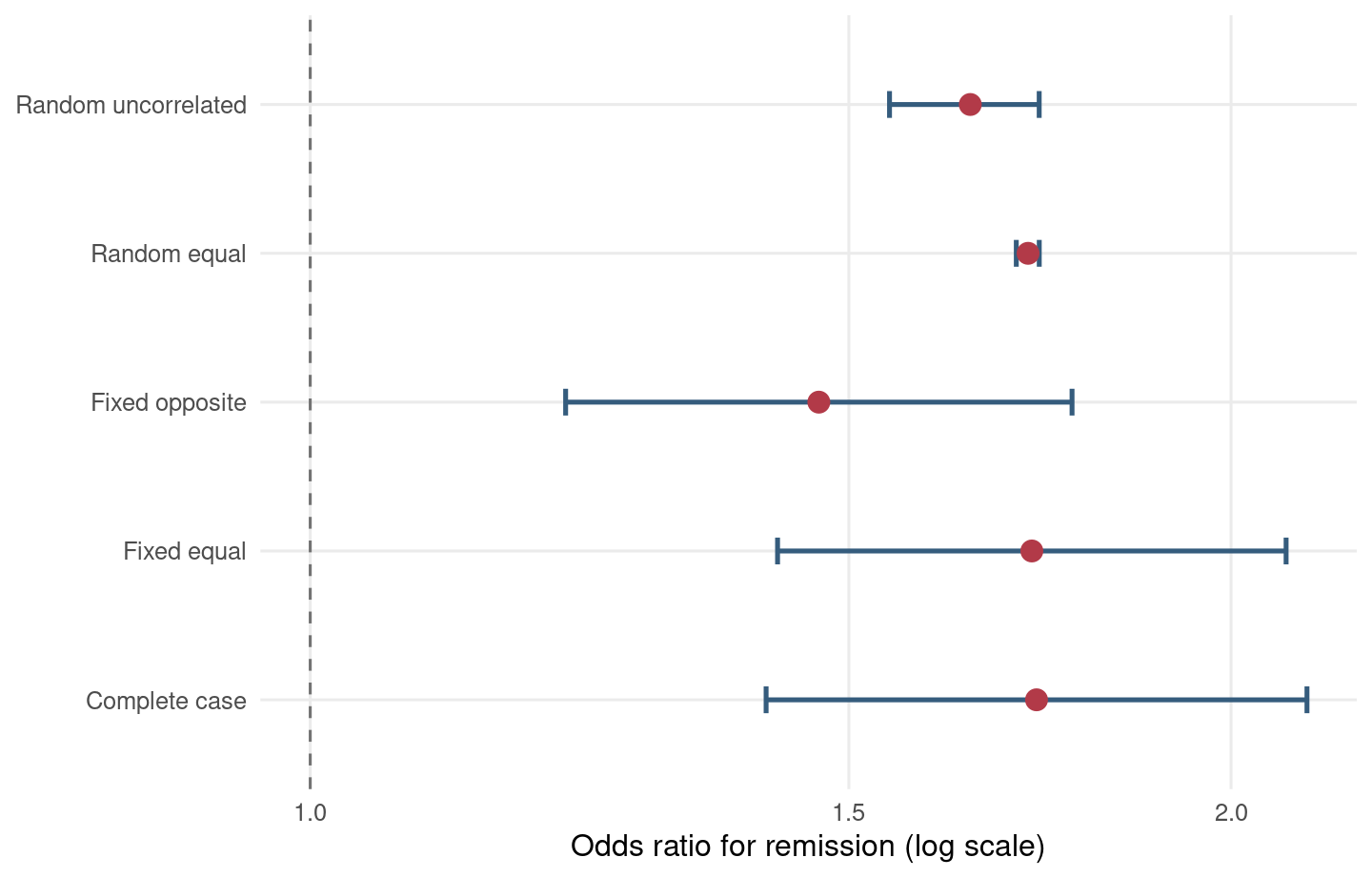
Complete case	1.728	1.409	2.118
Fixed equal	1.722	1.422	2.085
Fixed opposite	1.466	1.212	1.774
Random equal	1.717	1.701	1.731
Random uncorrelated	1.644	1.547	1.731

Code

ggplot(sensitivity_summary, aes(x = or, y = strategy)) +
  geom_vline(xintercept = 1, linetype = "dashed", color = "grey45") +
  geom_errorbar(aes(xmin = or_low, xmax = or_high), orientation = "y",
                width = 0.18, color = "#355C7D", linewidth = 0.9) +
  geom_point(size = 3.5, color = "#B23A48") +
  scale_x_log10(breaks = c(0.5, 1, 1.5, 2, 3)) +
  labs(x = "Odds ratio for remission (log scale)", y = NULL) +
  theme_minimal(base_size = 12) +
  theme(panel.grid.minor = element_blank())

Figure 6.1: 不同遺漏結局資料假設下的敏感度分析。

若所有合理情境都維持 OR > 1，結論較穩健；若 fixed opposite 或 random uncorrelated 讓區間跨過 1，表示失訪者假設會影響結論。這不是壞消息，而是誠實消息。

6.5 遺漏精確度

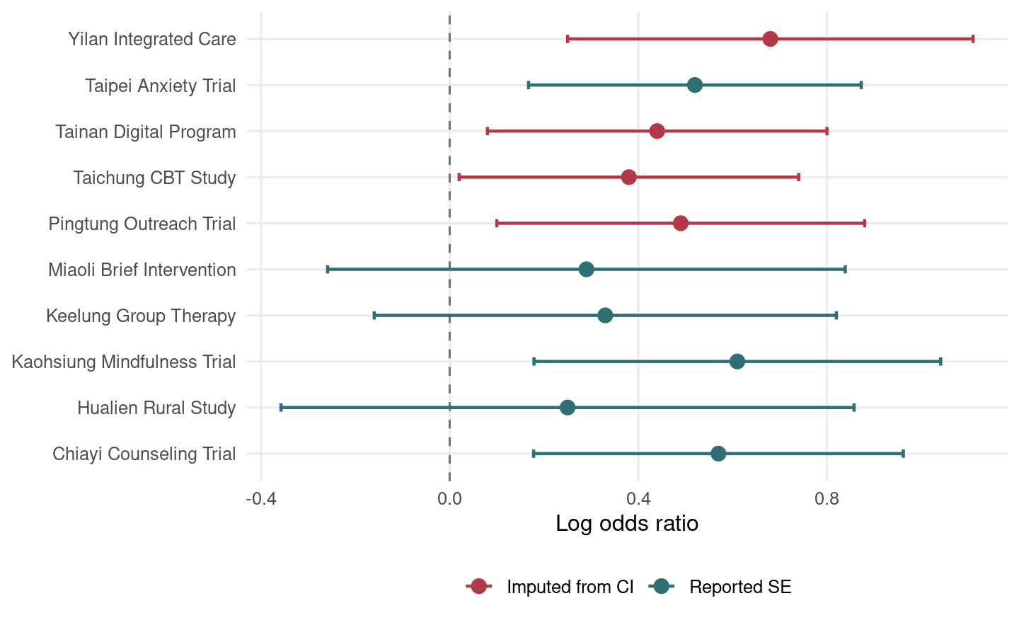
遺漏精確度 (missing precision) 指研究有報告效果估計，但缺少標準誤 (standard error, SE)、變異數或樣本數。若有 95% 信賴區間 (confidence interval, CI)，常可反推 SE：

\[ SE = \frac{\text{upper}-\text{lower}}{2\times1.96} \]

這裡的 upper 與 lower 必須和效果量在同一尺度；OR 應先轉成 log OR。

Code

precision <- tibble::tibble(
  study = c("Taipei Anxiety Trial", "Taichung CBT Study",
            "Kaohsiung Mindfulness Trial", "Tainan Digital Program",
            "Hualien Rural Study", "Chiayi Counseling Trial",
            "Keelung Group Therapy", "Pingtung Outreach Trial",
            "Miaoli Brief Intervention", "Yilan Integrated Care"),
  log_or = c(0.52, 0.38, 0.61, 0.44, 0.25, 0.57, 0.33, 0.49, 0.29, 0.68),
  se = c(0.18, NA, 0.22, NA, 0.31, 0.20, 0.25, NA, 0.28, NA),
  ci_low = c(0.17, 0.02, 0.18, 0.08, -0.36, 0.18, -0.16, 0.10, -0.26, 0.25),
  ci_high = c(0.87, 0.74, 1.04, 0.80, 0.86, 0.96, 0.82, 0.88, 0.84, 1.11),
  n_total = c(420, 360, 300, 340, 180, 280, 240, 390, 210, 320)
)

precision_completed <- precision |>
  mutate(
    se_from_ci = (ci_high - ci_low) / (2 * 1.96),
    se_imputed = if_else(is.na(se), se_from_ci, se),
    source = if_else(is.na(se), "Imputed from CI", "Reported SE"),
    vi = se_imputed^2
  )

kable(precision_completed, digits = 3)

study	log_or	se	ci_low	ci_high	n_total	se_from_ci	se_imputed	source	vi
Taipei Anxiety Trial	0.52	0.18	0.17	0.87	420	0.179	0.180	Reported SE	0.032
Taichung CBT Study	0.38	NA	0.02	0.74	360	0.184	0.184	Imputed from CI	0.034
Kaohsiung Mindfulness Trial	0.61	0.22	0.18	1.04	300	0.219	0.220	Reported SE	0.048
Tainan Digital Program	0.44	NA	0.08	0.80	340	0.184	0.184	Imputed from CI	0.034
Hualien Rural Study	0.25	0.31	-0.36	0.86	180	0.311	0.310	Reported SE	0.096
Chiayi Counseling Trial	0.57	0.20	0.18	0.96	280	0.199	0.200	Reported SE	0.040
Keelung Group Therapy	0.33	0.25	-0.16	0.82	240	0.250	0.250	Reported SE	0.062
Pingtung Outreach Trial	0.49	NA	0.10	0.88	390	0.199	0.199	Imputed from CI	0.040
Miaoli Brief Intervention	0.29	0.28	-0.26	0.84	210	0.281	0.280	Reported SE	0.078
Yilan Integrated Care	0.68	NA	0.25	1.11	320	0.219	0.219	Imputed from CI	0.048

Code

ggplot(precision_completed, aes(x = log_or, y = study)) +
  geom_vline(xintercept = 0, linetype = "dashed", color = "grey45") +
  geom_errorbar(aes(xmin = log_or - 1.96 * se_imputed,
                    xmax = log_or + 1.96 * se_imputed,
                    color = source),
                orientation = "y", width = 0.18, linewidth = 0.8) +
  geom_point(aes(color = source), size = 3.2) +
  scale_color_manual(values = c("Reported SE" = "#2F6F73", "Imputed from CI" = "#B23A48")) +
  labs(x = "Log odds ratio", y = NULL, color = NULL) +
  theme_minimal(base_size = 12) +
  theme(legend.position = "bottom", panel.grid.minor = element_blank())

Figure 6.2: 以信賴區間反推標準誤後納入分析的研究。

6.5.1 多重插補方法

多重插補 (multiple imputation) 不只填一個值，而是產生多個合理完整資料集，分別分析後再合併。本章使用 mice 套件的 predictive mean matching 來插補缺少的 SE，接著用 Rubin’s rules 合併統合分析結果。

Code

set.seed(20260630)
m <- 30
mi_input <- precision_completed |>
  select(log_or, se, n_total)
mi_method <- make.method(mi_input)
mi_method[c("log_or", "n_total")] <- ""
mi_method["se"] <- "pmm"
mi_predictors <- make.predictorMatrix(mi_input)
mi_predictors[,] <- 0
mi_predictors["se", c("log_or", "n_total")] <- 1
mi_fit <- mice(
  mi_input,
  m = m,
  maxit = 10,
  method = mi_method,
  predictorMatrix = mi_predictors,
  printFlag = FALSE,
  seed = 20260630
)

mi_results <- bind_rows(lapply(seq_len(m), function(i) {
  completed <- complete(mi_fit, action = i) |>
    mutate(vi_mi = se^2)
  fit <- rma.uni(yi = log_or, vi = vi_mi, data = completed, method = "DL")
  tibble::tibble(
    imputation = i,
    log_or = as.numeric(fit$b[1]),
    variance = fit$se^2
  )
}))

pooled_log_or <- mean(mi_results$log_or)
within_var <- mean(mi_results$variance)
between_var <- var(mi_results$log_or)
total_var <- within_var + (1 + 1 / m) * between_var
mi_summary <- tibble::tibble(
  method = "Multiple imputation of missing SE",
  log_or = pooled_log_or,
  se = sqrt(total_var),
  lower = pooled_log_or - 1.96 * sqrt(total_var),
  upper = pooled_log_or + 1.96 * sqrt(total_var),
  or = exp(log_or),
  or_low = exp(lower),
  or_high = exp(upper)
)

kable(mi_summary, digits = 3)

method	log_or	se	lower	upper	or	or_low	or_high
Multiple imputation of missing SE	0.479	0.072	0.338	0.62	1.615	1.402	1.86

其中 within variance 是各插補資料集分析變異的平均，between variance 是插補資料集間估計值的變異；兩者合併後就是 Rubin’s rules 的核心精神。若你的環境尚未安裝 mice，可執行：

Code

install.packages("mice")

6.5.2 遺漏受試者人數

遺漏受試者人數 (missing participant numbers) 有時出現在摘要表：研究報告事件數，卻沒有清楚列出各組分母。若已知總隨機分派人數與分派比例，可做合理推估；若不確定，應做敏感度分析。

Code

missing_n <- tibble::tibble(
  study = c("Registry A", "Registry B", "Registry C"),
  event_tx = c(32, 45, 28),
  event_ctrl = c(41, 60, 34),
  total_tx_reported = c(NA, 520, NA),
  total_ctrl_reported = c(500, NA, NA),
  total_randomised = c(980, 1040, 760)
) |>
  mutate(
    total_tx_imputed = if_else(is.na(total_tx_reported),
                               round(total_randomised / 2),
                               total_tx_reported),
    total_ctrl_imputed = if_else(is.na(total_ctrl_reported),
                                 total_randomised - total_tx_imputed,
                                 total_ctrl_reported)
  )

kable(missing_n, digits = 0)

study	event_tx	event_ctrl	total_tx_reported	total_ctrl_reported	total_randomised	total_tx_imputed	total_ctrl_imputed
Registry A	32	41	NA	500	980	490	500
Registry B	45	60	520	NA	1040	520	520
Registry C	28	34	NA	NA	760	380	380

請把這類推估寫清楚。透明比假裝精確重要很多，尤其在統合分析裡。

6.6 R 工作流程與套件提醒

本章完整 R 腳本儲存在 scripts/chapter6.R。你可以在專案根目錄執行：

Code

/usr/bin/Rscript scripts/chapter6.R

本章可執行內容使用 metafor、ggplot2、dplyr、knitr；若要進行正式多重插補，也可使用 mice。目前本機皆已安裝。若你的環境缺少 mice，可執行：

Code

install.packages("mice")

6.7 小結

遺漏資料不是統計分析的邊角料，而是證據可信度的一部分。完整案例分析很方便，但可能偏倚。Study-level adjustment 與敏感度分析可以檢查結論是否依賴特定失訪假設；遺漏精確度可以從信賴區間反推，或用多重插補處理不確定性；遺漏受試者人數則需要透明推估與敏感度分析。

下一章會進入 multivariate meta-analysis。到那裡，我們不只面對一個結局或一個效果量，而是多個相關結果一起出現。統計桌面又會熱鬧一些，但我們會繼續一塊一塊拼起來。

6.8 Glossary

中文	English
遺漏資料	missing data
遺漏結局資料	missing outcome data
完整案例分析	complete-case analysis
敏感度分析	sensitivity analysis
Study-level adjustment	study-level adjustment
Informative missingness odds ratio	informative missingness odds ratio, IMOR
Fixed equal	fixed equal
Fixed opposite	fixed opposite
Random equal	random equal
Random uncorrelated	random uncorrelated
勝算比	odds ratio, OR
遺漏精確度	missing precision
標準誤	standard error, SE
信賴區間	confidence interval, CI
多重插補	multiple imputation
Rubin’s rules	Rubin’s rules
遺漏受試者人數	missing participant numbers
隨機效應模型	random-effects model
研究間變異	between-study variance