多變量統合分析 (Multivariate Meta-Analysis)

一次處理多個結局,讓相關性不要在角落裝沒事

7.1 本章學習目標

讀完本章後,你應該能夠:

  1. 說明多變量統合分析 (multivariate meta-analysis) 與單變量統合分析 (univariate meta-analysis) 的差異。
  2. 建立同一研究內多個效果量的共變異矩陣 (variance-covariance matrix)。
  3. 使用固定效應模型 (fixed-effect model) 同時合併多個結局。
  4. 處理不平衡資料 (unbalanced data),也就是不同研究回報不同結局。
  5. 使用 metafor::rma.mv() 配適隨機效應模型 (random-effects model)。

到目前為止,我們多半一次處理一種結局。但臨床研究常常很貪心,這其實是好事:一個糖尿病數位照護試驗可能同時報告 HbA1c、體重、血壓、生活品質與低血糖事件。若我們把每個結局完全分開分析,就會忽略同一研究中結局之間的相關性。

多變量統合分析的精神是:多個結局可以一起分析,而且要承認它們彼此相關。統計模型在這裡很像一位細心的共同作者,提醒我們:「同一篇研究的兩個結果,不是兩個完全陌生人。」

本章使用的臨床情境是:數位糖尿病照護是否能改善 HbA1c 與體重。效果量都是平均差 (mean difference, MD),數值小於 0 代表介入組改善較多。

7.2 固定效應模型

多變量固定效應模型 (multivariate fixed-effect model) 假設每個結局各有一個共同真實效果,研究之間的差異來自抽樣誤差。和單變量模型不同的是,我們需要描述同一研究內不同結局效果量的共變異。

若一篇研究同時報告 HbA1c 與體重,其效果量向量可寫成:

\[ \hat{\boldsymbol{\theta}}_i = \begin{pmatrix} \hat{\theta}_{i,HbA1c}\\ \hat{\theta}_{i,Weight} \end{pmatrix} \]

對應的研究內共變異矩陣為:

\[ \mathbf{V}_i = \begin{pmatrix} SE_{i,HbA1c}^2 & \rho SE_{i,HbA1c}SE_{i,Weight}\\ \rho SE_{i,HbA1c}SE_{i,Weight} & SE_{i,Weight}^2 \end{pmatrix} \]

其中 \(\rho\) 是同一研究內兩個效果量的相關係數。本章用 \(\rho=0.45\) 作為教學假設。實務上,若原文沒有提供相關性,常需要做敏感度分析。

Code
make_within_study_v <- function(dat, rho = 0.45) {
  dat <- dat |>
    mutate(.study_order = factor(study, levels = unique(study))) |>
    arrange(.study_order)
  blocks <- lapply(split(dat, dat$.study_order), function(x) {
    v <- diag(x$se^2, nrow = nrow(x))
    if (nrow(x) > 1) {
      for (i in seq_len(nrow(x))) {
        for (j in seq_len(nrow(x))) {
          if (i != j) {
            v[i, j] <- rho * x$se[i] * x$se[j]
          }
        }
      }
    }
    v
  })
  bldiag(blocks)
}

coef_tbl <- function(fit, model) {
  out <- as.data.frame(coef(summary(fit)))
  out$outcome <- gsub("^outcome", "", rownames(out))
  tibble::as_tibble(out) |>
    transmute(
      model = model,
      outcome,
      estimate,
      se,
      lower = ci.lb,
      upper = ci.ub
    )
}
Code
digital <- tibble::tibble(
  study = c("Taipei Diabetes App", "Taipei Diabetes App",
            "Taichung Coaching Trial", "Taichung Coaching Trial",
            "Kaohsiung CGM Study", "Kaohsiung CGM Study",
            "Tainan Primary Care", "Tainan Primary Care",
            "Hualien Rural Program", "Hualien Rural Program",
            "Chiayi Pharmacist Trial", "Chiayi Pharmacist Trial",
            "Keelung Nurse Support", "Keelung Nurse Support",
            "Pingtung Community Trial", "Pingtung Community Trial",
            "Miaoli Brief Messaging",
            "Yilan Integrated Platform", "Yilan Integrated Platform"),
  outcome = c("HbA1c", "Weight",
              "HbA1c", "Weight",
              "HbA1c", "Weight",
              "HbA1c", "Weight",
              "HbA1c", "Weight",
              "HbA1c", "Weight",
              "HbA1c", "Weight",
              "HbA1c", "Weight",
              "HbA1c",
              "HbA1c", "Weight"),
  yi = c(-0.42, -1.8,
         -0.35, -1.7,
         -0.72, -2.7,
         -0.31, -1.3,
         -0.12, -1.4,
         -0.47, -0.4,
         -0.28, -1.8,
         -0.05, -0.2,
         -0.25,
         -0.66, -2.5),
  se = c(0.13, 0.55,
         0.14, 0.50,
         0.16, 0.70,
         0.12, 0.45,
         0.15, 0.60,
         0.14, 0.52,
         0.13, 0.48,
         0.17, 0.62,
         0.16,
         0.15, 0.58),
  risk_of_bias = c("Some concerns", "Some concerns",
                   "Low", "Low",
                   "Low", "Low",
                   "Some concerns", "Some concerns",
                   "High", "High",
                   "Some concerns", "Some concerns",
                   "Some concerns", "Some concerns",
                   "High", "High",
                   "High",
                   "Low", "Low")
) |>
  mutate(
    outcome = factor(outcome, levels = c("HbA1c", "Weight")),
    vi = se^2,
    ci_low = yi - 1.96 * se,
    ci_high = yi + 1.96 * se
  )

kable(
  digital |>
    transmute(研究 = study, 結局 = outcome, `MD` = yi, `SE` = se,
              `95% CI` = sprintf("%.2f to %.2f", ci_low, ci_high),
              `偏差風險` = risk_of_bias),
  digits = 2
)
研究 結局 MD SE 95% CI 偏差風險
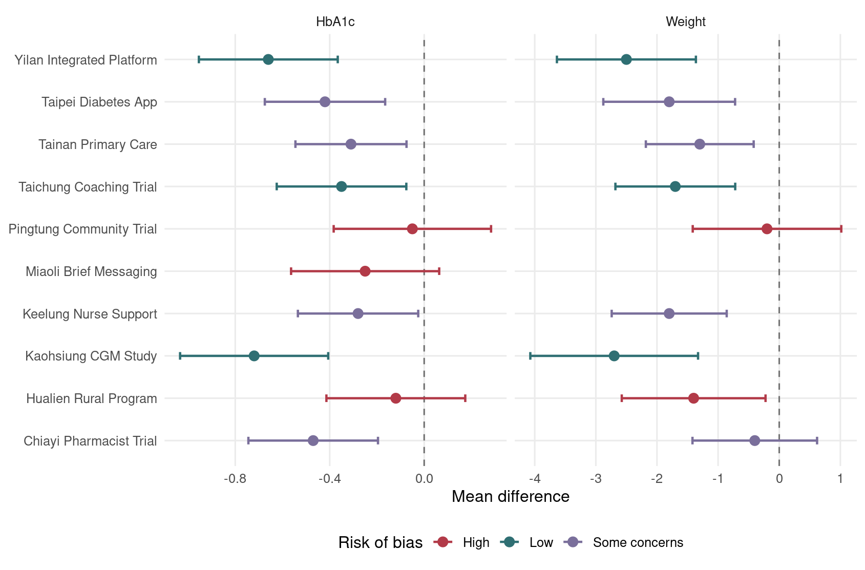
Taipei Diabetes App HbA1c -0.42 0.13 -0.67 to -0.17 Some concerns
Taipei Diabetes App Weight -1.80 0.55 -2.88 to -0.72 Some concerns
Taichung Coaching Trial HbA1c -0.35 0.14 -0.62 to -0.08 Low
Taichung Coaching Trial Weight -1.70 0.50 -2.68 to -0.72 Low
Kaohsiung CGM Study HbA1c -0.72 0.16 -1.03 to -0.41 Low
Kaohsiung CGM Study Weight -2.70 0.70 -4.07 to -1.33 Low
Tainan Primary Care HbA1c -0.31 0.12 -0.55 to -0.07 Some concerns
Tainan Primary Care Weight -1.30 0.45 -2.18 to -0.42 Some concerns
Hualien Rural Program HbA1c -0.12 0.15 -0.41 to 0.17 High
Hualien Rural Program Weight -1.40 0.60 -2.58 to -0.22 High
Chiayi Pharmacist Trial HbA1c -0.47 0.14 -0.74 to -0.20 Some concerns
Chiayi Pharmacist Trial Weight -0.40 0.52 -1.42 to 0.62 Some concerns
Keelung Nurse Support HbA1c -0.28 0.13 -0.53 to -0.03 Some concerns
Keelung Nurse Support Weight -1.80 0.48 -2.74 to -0.86 Some concerns
Pingtung Community Trial HbA1c -0.05 0.17 -0.38 to 0.28 High
Pingtung Community Trial Weight -0.20 0.62 -1.42 to 1.02 High
Miaoli Brief Messaging HbA1c -0.25 0.16 -0.56 to 0.06 High
Yilan Integrated Platform HbA1c -0.66 0.15 -0.95 to -0.37 Low
Yilan Integrated Platform Weight -2.50 0.58 -3.64 to -1.36 Low
Code
v_mat <- make_within_study_v(digital, rho = 0.45)

fit_mv_fe <- rma.mv(
  yi,
  V = v_mat,
  mods = ~ outcome - 1,
  data = digital,
  method = "FE"
)

fixed_summary <- coef_tbl(fit_mv_fe, "Multivariate fixed effect")

kable(
  fixed_summary |>
    transmute(模型 = model, 結局 = outcome, `合併 MD` = estimate,
              `SE` = se, `95% CI` = sprintf("%.2f to %.2f", lower, upper)),
  digits = 3
)
模型 結局 合併 MD SE 95% CI
Multivariate fixed effect HbA1c -0.363 0.045 -0.45 to -0.27
Multivariate fixed effect Weight -1.483 0.179 -1.83 to -1.13

固定效應模型顯示數位照護與 HbA1c、體重下降皆有關。請記得,這裡的重點不是「一次跑兩個模型比較省時間」,而是同時使用兩個結局的資訊與相關性。

7.3 處理不平衡資料

不平衡資料 (unbalanced data) 指不同研究回報的結局不完全相同。本例中,Miaoli Brief Messaging 只回報 HbA1c,沒有回報體重。多變量模型可以納入這類研究,而不是把它整篇丟掉。這點很重要,因為丟資料很容易,丟掉之後造成偏差也很容易。

Code
unbalanced <- digital |>
  count(study, name = "reported_outcomes") |>
  mutate(pattern = if_else(reported_outcomes == 2, "Both outcomes", "HbA1c only"))

kable(
  unbalanced,
  col.names = c("研究", "回報結局數", "資料型態"),
  digits = 0
)
研究 回報結局數 資料型態
Chiayi Pharmacist Trial 2 Both outcomes
Hualien Rural Program 2 Both outcomes
Kaohsiung CGM Study 2 Both outcomes
Keelung Nurse Support 2 Both outcomes
Miaoli Brief Messaging 1 HbA1c only
Pingtung Community Trial 2 Both outcomes
Taichung Coaching Trial 2 Both outcomes
Tainan Primary Care 2 Both outcomes
Taipei Diabetes App 2 Both outcomes
Yilan Integrated Platform 2 Both outcomes
Code
ggplot(digital, aes(x = yi, y = study)) +
  geom_vline(xintercept = 0, linetype = "dashed", color = "grey45") +
  geom_errorbar(aes(xmin = ci_low, xmax = ci_high, color = risk_of_bias),
                orientation = "y", width = 0.18, linewidth = 0.8) +
  geom_point(aes(color = risk_of_bias), size = 3) +
  facet_wrap(~ outcome, scales = "free_x") +
  scale_color_manual(values = c("Low" = "#2F6F73", "Some concerns" = "#7A6F9B", "High" = "#B23A48")) +
  labs(x = "Mean difference", y = NULL, color = "Risk of bias") +
  theme_minimal(base_size = 12) +
  theme(legend.position = "bottom", panel.grid.minor = element_blank())

Figure 7.1: 數位糖尿病照護研究中 HbA1c 與體重兩個結局的研究層級效果量。

如果只做兩個單變量分析,仍然可以納入各結局可用資料;但多變量模型進一步利用同一研究內結局相關性。這在結局缺漏不完全隨機時尤其有價值。

7.4 隨機效應模型

隨機效應多變量模型 (multivariate random-effects model) 允許不同研究在每個結局上有不同真實效果,也允許這些真實效果之間相關。模型可寫成:

\[ \hat{\boldsymbol{\theta}}_i = \boldsymbol{\mu} + \mathbf{u}_i + \mathbf{e}_i \]

其中 \(\mathbf{e}_i\) 是研究內誤差,\(\mathbf{u}_i\) 是研究間隨機效應。若 HbA1c 效果大的研究也常有較大體重效果,研究間隨機效應就可能呈現正相關。

7.4.1 配適隨機效應模型

Code
fit_mv_re <- rma.mv(
  yi,
  V = v_mat,
  mods = ~ outcome - 1,
  random = ~ outcome | study,
  struct = "UN",
  data = digital,
  method = "REML"
)

random_summary <- coef_tbl(fit_mv_re, "Multivariate random effects")

univariate_summary <- digital |>
  group_by(outcome) |>
  group_modify(\(.x, .y) {
    fit <- rma.uni(yi = yi, vi = vi, data = .x, method = "REML")
    tibble::tibble(
      estimate = as.numeric(fit$b[1]),
      se = fit$se,
      lower = fit$ci.lb,
      upper = fit$ci.ub,
      tau2 = fit$tau2,
      i2 = fit$I2
    )
  }) |>
  ungroup() |>
  mutate(model = "Separate univariate")

summary_all <- bind_rows(
  univariate_summary |>
    transmute(model, outcome = as.character(outcome), estimate, se, lower, upper),
  fixed_summary,
  random_summary
)

kable(
  summary_all |>
    transmute(模型 = model, 結局 = outcome, `合併 MD` = estimate,
              `SE` = se, `95% CI` = sprintf("%.2f to %.2f", lower, upper)),
  digits = 3
)
模型 結局 合併 MD SE 95% CI
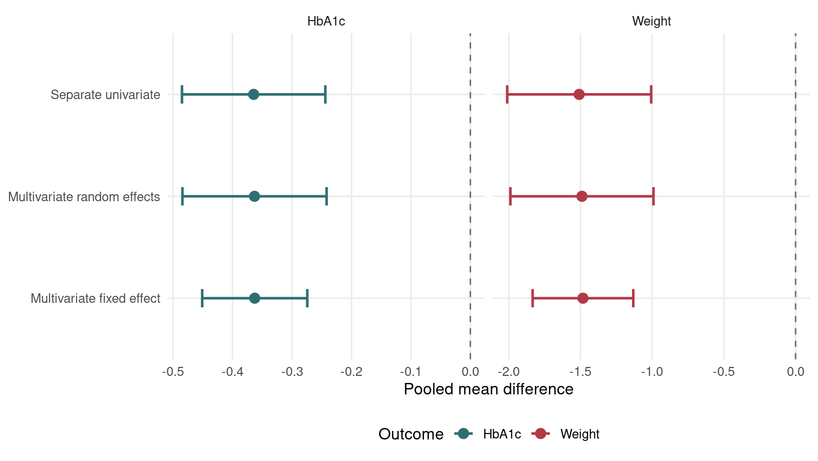
Separate univariate HbA1c -0.364 0.062 -0.49 to -0.24
Separate univariate Weight -1.509 0.256 -2.01 to -1.01
Multivariate fixed effect HbA1c -0.363 0.045 -0.45 to -0.27
Multivariate fixed effect Weight -1.483 0.179 -1.83 to -1.13
Multivariate random effects HbA1c -0.363 0.062 -0.48 to -0.24
Multivariate random effects Weight -1.490 0.255 -1.99 to -0.99
Code
random_params <- tibble::tibble(
  parameter = c("tau-squared level 1", "tau-squared level 2", "rho"),
  value = c(fit_mv_re$tau2, fit_mv_re$rho)
)

kable(random_params, col.names = c("參數", "估計值"), digits = 3)
參數 估計值
tau-squared level 1 0.018
tau-squared level 2 0.300
rho 0.755

tau-squared 描述研究間變異 (between-study variance),rho 描述兩個結局的研究間隨機效應相關。若 rho 為正,代表在 HbA1c 效果較大的研究中,體重效果也傾向較大。請注意,研究數不多時,這些變異與相關參數可能估得不穩,所以解讀要溫柔一點,不要把它們當成石碑。

Code
ggplot(summary_all, aes(x = estimate, y = model)) +
  geom_vline(xintercept = 0, linetype = "dashed", color = "grey45") +
  geom_errorbar(aes(xmin = lower, xmax = upper, color = outcome),
                orientation = "y", width = 0.18, linewidth = 0.9,
                position = position_dodge(width = 0.55)) +
  geom_point(aes(color = outcome), size = 3.2,
             position = position_dodge(width = 0.55)) +
  facet_wrap(~ outcome, scales = "free_x") +
  scale_color_manual(values = c("HbA1c" = "#2F6F73", "Weight" = "#B23A48")) +
  labs(x = "Pooled mean difference", y = NULL, color = "Outcome") +
  theme_minimal(base_size = 12) +
  theme(legend.position = "bottom", panel.grid.minor = element_blank())

Figure 7.2: 單變量分析、多變量固定效應模型與多變量隨機效應模型的合併估計比較。

7.5 討論

多變量統合分析適合用在多個相關結局、同一研究報告多個效果量、或研究回報結局不完全一致的情境。它的優點包括:

  • 可以保留不平衡資料,不必只分析完整回報所有結局的研究。
  • 可以納入研究內相關性,避免把同一研究的多個結局當成完全獨立。
  • 可以估計研究間不同結局效果的相關性。

但它也有代價。第一,模型需要更多假設,尤其是研究內相關性。第二,研究數少時,變異與相關參數可能很不穩。第三,輸出比單變量模型更難解釋,報告時要清楚說明資料結構、共變異矩陣如何建立、相關性假設如何處理。

實務上,建議至少做一個研究內相關係數的敏感度分析。例如把 \(\rho\) 設成 0、0.3、0.6,檢查合併估計是否穩定。如果結果對 \(\rho\) 很敏感,就要在討論中明確寫出來。統計模型可以優雅,但誠實更重要。

7.6 R 工作流程與套件提醒

本章完整 R 腳本儲存在 scripts/chapter7.R。你可以在專案根目錄執行:

Code
/usr/bin/Rscript scripts/chapter7.R

本章使用 metaforggplot2dplyrknitr,目前本機皆已安裝。rma.mv() 是本章的主角,負責配適多層次與多變量統合分析模型。

7.7 Glossary

中文 English
多變量統合分析 multivariate meta-analysis
單變量統合分析 univariate meta-analysis
平均差 mean difference, MD
共變異矩陣 variance-covariance matrix
固定效應模型 fixed-effect model
隨機效應模型 random-effects model
不平衡資料 unbalanced data
研究內相關性 within-study correlation
研究內誤差 within-study error
研究間隨機效應 between-study random effects
研究間變異 between-study variance
限制最大概似法 restricted maximum likelihood, REML
隨機效應相關 random-effects correlation
敏感度分析 sensitivity analysis