診斷性試驗準確性研究的統合分析 (Meta-Analysis of Diagnostic Test Accuracy Studies)

敏感度、特異度與 ROC 曲線：診斷研究的雙人舞

9.1 本章學習目標

讀完本章後，你應該能夠：

說明診斷準確度研究 (diagnostic test accuracy study, DTA study) 的特殊挑戰。
計算敏感度 (sensitivity)、特異度 (specificity)、診斷勝算比 (diagnostic odds ratio, DOR) 與似然比 (likelihood ratio)。
繪製敏感度與特異度散佈圖，以及 summary ROC curve。
說明 hierarchical model 與 bivariate model 的概念。
使用 mada 配適 Reitsma bivariate diagnostic accuracy model，並理解 meta4diag 的 Bayesian 延伸用途。

治療研究通常問：「這個介入有沒有效？」診斷研究則更像在問：「這個檢查有多會抓到真正有病的人，又有多會放過真正沒病的人？」這裡沒有單一結局可以偷懶，因為敏感度與特異度常常一個上升、另一個下降。診斷統合分析就是在這種拉扯中找平衡。

本章使用的臨床情境是：急診高敏感度 troponin 快速檢測用於診斷急性心肌梗塞。參考標準 (reference standard) 是心臟科醫師根據完整臨床資料與序列 troponin 判定的最終診斷。

9.2 診斷準確度研究的特殊挑戰

診斷準確度研究與治療試驗不同，常見挑戰包括：

閾值效應 (threshold effect)：不同研究使用不同檢測 cut-off，會同時影響 sensitivity 與 specificity。
參考標準偏倚 (reference standard bias)：若 gold standard 本身不完美，準確度估計會被影響。
驗證偏倚 (verification bias)：若只有部分病人接受參考標準檢查，可能造成偏差。
疾病盛行率與 spectrum effect：病人嚴重度、共病與照護場域會影響檢測表現。

診斷研究不是單純把 TP、FP、FN、TN 加一加就好。就像急診值班，數字看起來很快，但背後永遠有脈絡。

Code

logit <- function(p) log(p / (1 - p))
inv_logit <- function(x) exp(x) / (1 + exp(x))

dta_measures <- function(dat, correction = 0.5) {
  dat |>
    mutate(
      tp_c = if_else(tp == 0 | fn == 0 | fp == 0 | tn == 0, tp + correction, as.numeric(tp)),
      fn_c = if_else(tp == 0 | fn == 0 | fp == 0 | tn == 0, fn + correction, as.numeric(fn)),
      fp_c = if_else(tp == 0 | fn == 0 | fp == 0 | tn == 0, fp + correction, as.numeric(fp)),
      tn_c = if_else(tp == 0 | fn == 0 | fp == 0 | tn == 0, tn + correction, as.numeric(tn)),
      sensitivity = tp_c / (tp_c + fn_c),
      specificity = tn_c / (tn_c + fp_c),
      fpr = 1 - specificity,
      ppv = tp_c / (tp_c + fp_c),
      npv = tn_c / (tn_c + fn_c),
      lr_pos = sensitivity / (1 - specificity),
      lr_neg = (1 - sensitivity) / specificity,
      dor = (tp_c * tn_c) / (fp_c * fn_c),
      log_dor = log(dor),
      se_log_dor = sqrt(1 / tp_c + 1 / fn_c + 1 / fp_c + 1 / tn_c),
      logit_sens = logit(sensitivity),
      vi_sens = 1 / tp_c + 1 / fn_c,
      logit_fpr = logit(fpr),
      vi_fpr = 1 / fp_c + 1 / tn_c
    )
}

make_v <- function(dat) {
  blocks <- lapply(seq_len(nrow(dat)), function(i) {
    matrix(c(dat$vi_sens[i], 0, 0, dat$vi_fpr[i]), nrow = 2)
  })
  bldiag(blocks)
}

Code

troponin <- tibble::tibble(
  study = c("Taipei ED Cohort", "Taichung Chest Pain Study",
            "Kaohsiung Rapid Rule-In", "Tainan Community Hospital",
            "Hualien Rural ED", "Chiayi Cardiology Unit",
            "Keelung Multicenter Study", "Pingtung Regional Hospital",
            "Miaoli Observation Unit", "Yilan Acute Care Study",
            "Nantou ED Registry", "Taitung Indigenous Health"),
  threshold = c(14, 14, 20, 14, 20, 14, 26, 20, 14, 26, 20, 14),
  tp = c(86, 64, 91, 58, 42, 77, 70, 48, 55, 63, 46, 39),
  fn = c(9, 8, 13, 11, 10, 7, 16, 12, 9, 17, 13, 8),
  fp = c(70, 55, 45, 64, 38, 62, 34, 42, 58, 30, 36, 44),
  tn = c(330, 285, 350, 260, 210, 305, 330, 240, 250, 310, 230, 205)
)

troponin_es <- dta_measures(troponin)

kable(
  troponin,
  col.names = c("研究", "Cut-off", "TP", "FN", "FP", "TN"),
  digits = 0
)

研究	Cut-off	TP	FN	FP	TN
Taipei ED Cohort	14	86	9	70	330
Taichung Chest Pain Study	14	64	8	55	285
Kaohsiung Rapid Rule-In	20	91	13	45	350
Tainan Community Hospital	14	58	11	64	260
Hualien Rural ED	20	42	10	38	210
Chiayi Cardiology Unit	14	77	7	62	305
Keelung Multicenter Study	26	70	16	34	330
Pingtung Regional Hospital	20	48	12	42	240
Miaoli Observation Unit	14	55	9	58	250
Yilan Acute Care Study	26	63	17	30	310
Nantou ED Registry	20	46	13	36	230
Taitung Indigenous Health	14	39	8	44	205

9.3 診斷準確度指標

9.3.1 敏感度與特異度

敏感度 (sensitivity) 是有病者中檢測陽性的比例：

\[ Sensitivity = \frac{TP}{TP+FN} \]

特異度 (specificity) 是無病者中檢測陰性的比例：

\[ Specificity = \frac{TN}{TN+FP} \]

Code

kable(
  troponin_es |>
    transmute(
      研究 = study,
      `Cut-off` = threshold,
      `Sensitivity` = sensitivity,
      `Specificity` = specificity,
      `PPV` = ppv,
      `NPV` = npv
    ),
  digits = 3
)

研究	Cut-off	Sensitivity	Specificity	PPV	NPV
Taipei ED Cohort	14	0.905	0.825	0.551	0.973
Taichung Chest Pain Study	14	0.889	0.838	0.538	0.973
Kaohsiung Rapid Rule-In	20	0.875	0.886	0.669	0.964
Tainan Community Hospital	14	0.841	0.802	0.475	0.959
Hualien Rural ED	20	0.808	0.847	0.525	0.955
Chiayi Cardiology Unit	14	0.917	0.831	0.554	0.978
Keelung Multicenter Study	26	0.814	0.907	0.673	0.954
Pingtung Regional Hospital	20	0.800	0.851	0.533	0.952
Miaoli Observation Unit	14	0.859	0.812	0.487	0.965
Yilan Acute Care Study	26	0.787	0.912	0.677	0.948
Nantou ED Registry	20	0.780	0.865	0.561	0.947
Taitung Indigenous Health	14	0.830	0.823	0.470	0.962

陽性預測值 (positive predictive value, PPV) 與陰性預測值 (negative predictive value, NPV) 很臨床，但會受疾病盛行率影響；sensitivity 與 specificity 較常作為 DTA meta-analysis 的主要建模對象。

9.3.2 其他指標：DOR 與似然比

陽性似然比 (positive likelihood ratio, LR+) 是 sensitivity 除以 false positive rate；陰性似然比 (negative likelihood ratio, LR-) 是 false negative rate 除以 specificity。

診斷勝算比 (diagnostic odds ratio, DOR) 可寫成：

\[ DOR = \frac{TP/FN}{FP/TN} = \frac{TP \times TN}{FP \times FN} \]

Code

kable(
  troponin_es |>
    transmute(
      研究 = study,
      `LR+` = lr_pos,
      `LR-` = lr_neg,
      `DOR` = dor
    ),
  digits = 2
)

研究	LR+	LR-	DOR
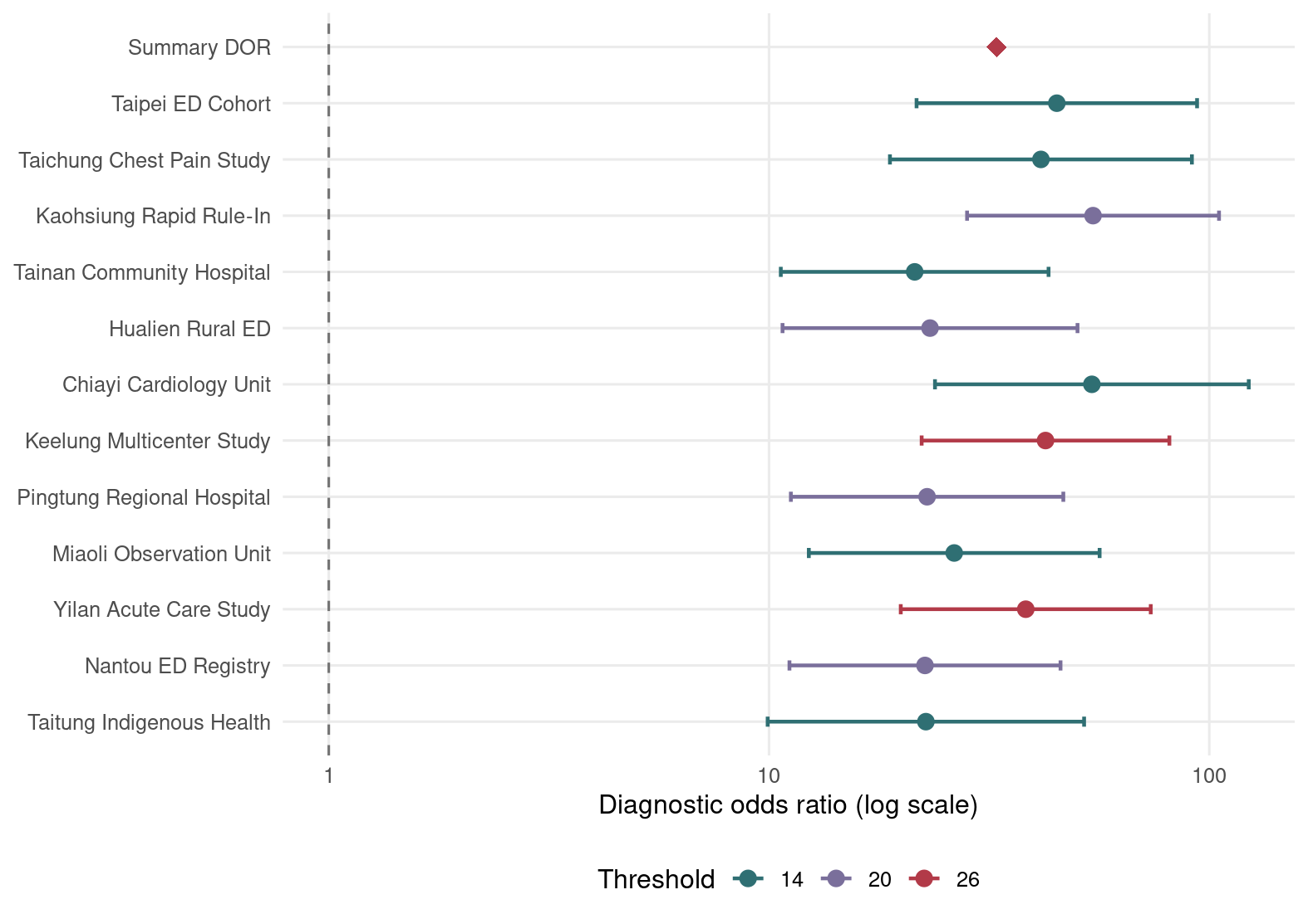
Taipei ED Cohort	5.17	0.11	45.05
Taichung Chest Pain Study	5.49	0.13	41.45
Kaohsiung Rapid Rule-In	7.68	0.14	54.44
Tainan Community Hospital	4.26	0.20	21.42
Hualien Rural ED	5.27	0.23	23.21
Chiayi Cardiology Unit	5.43	0.10	54.11
Keelung Multicenter Study	8.71	0.21	42.46
Pingtung Regional Hospital	5.37	0.23	22.86
Miaoli Observation Unit	4.56	0.17	26.34
Yilan Acute Care Study	8.92	0.23	38.29
Nantou ED Registry	5.76	0.25	22.61
Taitung Indigenous Health	4.70	0.21	22.71

DOR 把 sensitivity 與 specificity 壓成單一數字，方便但也有代價：兩個檢測可能 DOR 一樣，但一個 sensitivity 高、另一個 specificity 高，臨床用途完全不同。

9.3.3 連續型 marker 的檢測

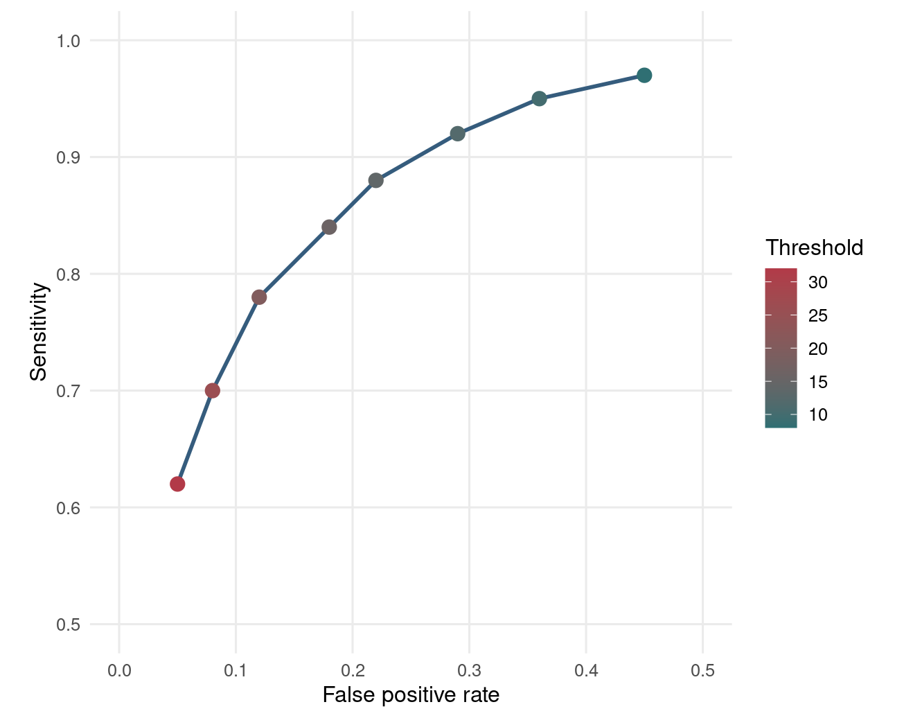
許多診斷檢查本質上是連續型 marker，例如 troponin、CRP、D-dimer 或 HbA1c。不同 cut-off 會產生不同 sensitivity 與 specificity，因此 ROC curve 很重要。

Code

marker <- tibble::tibble(
  threshold = c(8, 10, 12, 14, 16, 20, 26, 32),
  sensitivity = c(0.97, 0.95, 0.92, 0.88, 0.84, 0.78, 0.70, 0.62),
  specificity = c(0.55, 0.64, 0.71, 0.78, 0.82, 0.88, 0.92, 0.95)
)

ggplot(marker, aes(x = 1 - specificity, y = sensitivity)) +
  geom_path(color = "#355C7D", linewidth = 1) +
  geom_point(aes(color = threshold), size = 3.2) +
  scale_color_gradient(low = "#2F6F73", high = "#B23A48") +
  coord_equal(xlim = c(0, 0.5), ylim = c(0.5, 1)) +
  labs(x = "False positive rate", y = "Sensitivity", color = "Threshold") +
  theme_minimal(base_size = 12) +
  theme(panel.grid.minor = element_blank())

Figure 9.1: 連續型 troponin marker 在不同 cut-off 下形成的 ROC curve。

9.4 敏感度與特異度散佈圖

Code

ggplot(troponin_es, aes(x = 1 - specificity, y = sensitivity)) +
  geom_point(aes(size = tp + fn, color = factor(threshold)), alpha = 0.85) +
  scale_size_continuous(range = c(3, 8), guide = "none") +
  scale_color_manual(values = c("14" = "#2F6F73", "20" = "#7A6F9B", "26" = "#B23A48")) +
  coord_equal(xlim = c(0, 0.25), ylim = c(0.65, 1)) +
  labs(x = "False positive rate (1 - specificity)",
       y = "Sensitivity",
       color = "Threshold") +
  theme_minimal(base_size = 12) +
  theme(legend.position = "bottom", panel.grid.minor = element_blank())

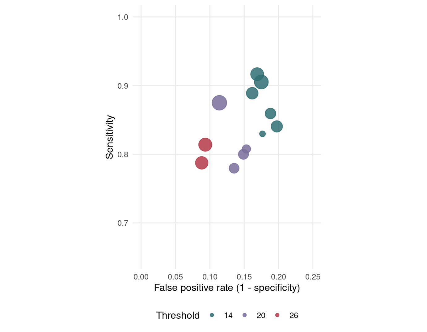
Figure 9.2: 各診斷準確度研究的 sensitivity 與 false positive rate 散佈圖。

若 cut-off 越低，通常 sensitivity 較高但 false positive rate 也較高。這就是診斷研究的日常拔河。

9.5 診斷準確度統合分析模型

9.5.1 Hierarchical model

Hierarchical model 是 DTA meta-analysis 的核心。它通常包含兩層：第一層描述每篇研究內 TP/FN/FP/TN 的抽樣變異，第二層描述研究間 sensitivity 與 specificity 的變異。常見模型包括 hierarchical summary ROC model (HSROC model) 與 bivariate model。

本章先用 metafor::rma.mv() 建立簡化 bivariate model，讓模型結構透明化；接著使用 DTA 專門套件 mada 的 reitsma() 配適正式 Reitsma bivariate model。meta4diag 也已安裝，適合進一步做 Bayesian diagnostic test accuracy meta-analysis。

9.5.2 Bivariate model

Bivariate model 同時建模 logit sensitivity 與 logit false positive rate，並允許兩者的研究間隨機效應相關。

Code

biv_dat <- bind_rows(
  troponin_es |>
    transmute(study, threshold, outcome = "Sensitivity", yi = logit_sens, vi = vi_sens),
  troponin_es |>
    transmute(study, threshold, outcome = "False positive rate", yi = logit_fpr, vi = vi_fpr)
) |>
  mutate(outcome = factor(outcome, levels = c("Sensitivity", "False positive rate"))) |>
  arrange(study, outcome)

v_mat <- make_v(troponin_es)

biv_random <- rma.mv(
  yi,
  V = v_mat,
  mods = ~ outcome - 1,
  random = ~ outcome | study,
  struct = "UN",
  data = biv_dat,
  method = "REML"
)

biv_summary <- as.data.frame(coef(summary(biv_random))) |>
  tibble::rownames_to_column("parameter") |>
  as_tibble() |>
  mutate(
    clinical_quantity = c("Summary sensitivity", "Summary false positive rate"),
    estimate_prob = inv_logit(estimate),
    lower_prob = inv_logit(ci.lb),
    upper_prob = inv_logit(ci.ub)
  )

kable(
  biv_summary |>
    transmute(項目 = clinical_quantity, 估計值 = estimate_prob,
              `95% CI` = sprintf("%.3f to %.3f", lower_prob, upper_prob)),
  digits = 3
)

項目	估計值	95% CI
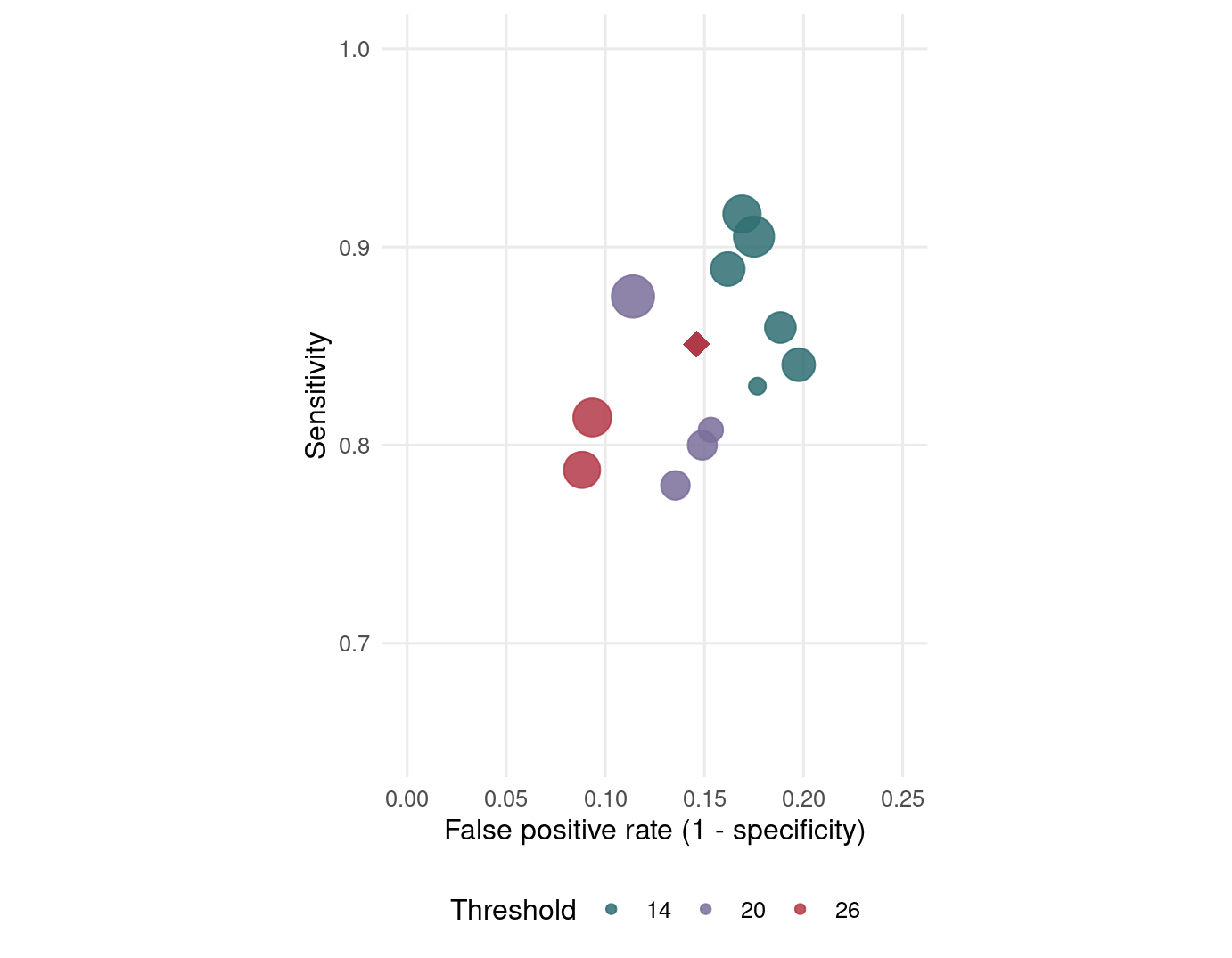
Summary sensitivity	0.851	0.821 to 0.877
Summary false positive rate	0.146	0.125 to 0.169

Code

summary_sens <- biv_summary$estimate_prob[biv_summary$clinical_quantity == "Summary sensitivity"]
summary_fpr <- biv_summary$estimate_prob[biv_summary$clinical_quantity == "Summary false positive rate"]
summary_spec <- 1 - summary_fpr
summary_point <- tibble::tibble(fpr = summary_fpr, sensitivity = summary_sens)

dor_fit <- rma.uni(yi = log_dor, sei = se_log_dor, data = troponin_es, method = "DL")

summary_measures <- tibble::tibble(
  quantity = c("Sensitivity", "Specificity", "Positive likelihood ratio",
               "Negative likelihood ratio", "Diagnostic odds ratio"),
  estimate = c(summary_sens, summary_spec,
               summary_sens / summary_fpr,
               (1 - summary_sens) / summary_spec,
               exp(as.numeric(dor_fit$b[1]))),
  lower = c(
    biv_summary$lower_prob[biv_summary$clinical_quantity == "Summary sensitivity"],
    1 - biv_summary$upper_prob[biv_summary$clinical_quantity == "Summary false positive rate"],
    NA_real_, NA_real_, exp(dor_fit$ci.lb)
  ),
  upper = c(
    biv_summary$upper_prob[biv_summary$clinical_quantity == "Summary sensitivity"],
    1 - biv_summary$lower_prob[biv_summary$clinical_quantity == "Summary false positive rate"],
    NA_real_, NA_real_, exp(dor_fit$ci.ub)
  )
)

kable(summary_measures, col.names = c("指標", "估計值", "95% CI 下限", "95% CI 上限"), digits = 3)

指標	估計值	95% CI 下限	95% CI 上限
Sensitivity	0.851	0.821	0.877
Specificity	0.854	0.831	0.875
Positive likelihood ratio	5.834	NA	NA
Negative likelihood ratio	0.175	NA	NA
Diagnostic odds ratio	32.851	26.650	40.496

Code

ggplot(troponin_es, aes(x = 1 - specificity, y = sensitivity)) +
  geom_point(aes(size = tp + fn, color = factor(threshold)), alpha = 0.85) +
  geom_point(data = summary_point, aes(x = fpr, y = sensitivity),
             inherit.aes = FALSE, shape = 18, size = 5, color = "#B23A48") +
  scale_size_continuous(range = c(3, 8), guide = "none") +
  scale_color_manual(values = c("14" = "#2F6F73", "20" = "#7A6F9B", "26" = "#B23A48")) +
  coord_equal(xlim = c(0, 0.25), ylim = c(0.65, 1)) +
  labs(x = "False positive rate (1 - specificity)",
       y = "Sensitivity",
       color = "Threshold") +
  theme_minimal(base_size = 12) +
  theme(legend.position = "bottom", panel.grid.minor = element_blank())

Figure 9.3: Bivariate model 的 summary sensitivity 與 false positive rate。紅色菱形為摘要估計。

9.5.3 使用 mada 的 Reitsma model

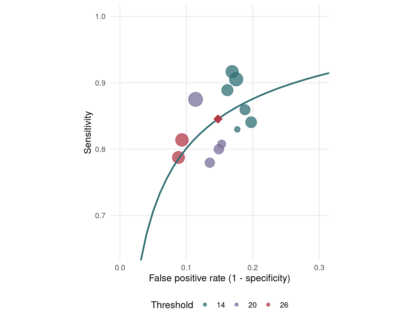
mada 是診斷準確度統合分析的專門套件。reitsma() 會以 logit sensitivity 與 logit false positive rate 配適 Reitsma bivariate model；這個模型與 HSROC model 在常用設定下有密切對應。

Code

troponin_mada <- troponin |>
  transmute(names = study, TP = tp, FN = fn, FP = fp, TN = tn)

mada_desc <- mada::madad(troponin_mada)
mada_fit <- mada::reitsma(troponin_mada)
mada_summary <- summary(mada_fit)
mada_coef <- as.data.frame(mada_summary$coefficients) |>
  tibble::rownames_to_column("parameter") |>
  as_tibble()
mada_auc <- mada::AUC(mada_fit)

mada_sens <- mada_coef$Estimate[mada_coef$parameter == "sensitivity"]
mada_sens_low <- mada_coef$`95%ci.lb`[mada_coef$parameter == "sensitivity"]
mada_sens_high <- mada_coef$`95%ci.ub`[mada_coef$parameter == "sensitivity"]
mada_fpr <- mada_coef$Estimate[mada_coef$parameter == "false pos. rate"]
mada_fpr_low <- mada_coef$`95%ci.lb`[mada_coef$parameter == "false pos. rate"]
mada_fpr_high <- mada_coef$`95%ci.ub`[mada_coef$parameter == "false pos. rate"]
mada_spec <- 1 - mada_fpr

mada_summary_measures <- tibble::tibble(
  quantity = c("Sensitivity", "Specificity", "Positive likelihood ratio",
               "Negative likelihood ratio", "Diagnostic odds ratio",
               "Area under the SROC curve"),
  estimate = c(mada_sens, mada_spec,
               mada_sens / mada_fpr,
               (1 - mada_sens) / mada_spec,
               (mada_sens / mada_fpr) / ((1 - mada_sens) / mada_spec),
               mada_auc$AUC),
  lower = c(mada_sens_low, 1 - mada_fpr_high, NA_real_, NA_real_, NA_real_, NA_real_),
  upper = c(mada_sens_high, 1 - mada_fpr_low, NA_real_, NA_real_, NA_real_, NA_real_)
)

kable(
  mada_summary_measures,
  col.names = c("指標", "估計值", "95% CI 下限", "95% CI 上限"),
  digits = 3
)

指標	估計值	95% CI 下限	95% CI 上限
Sensitivity	0.845	0.816	0.871
Specificity	0.852	0.830	0.872
Positive likelihood ratio	5.725	NA	NA
Negative likelihood ratio	0.181	NA	NA
Diagnostic odds ratio	31.575	NA	NA
Area under the SROC curve	0.909	NA	NA

Code

mada_random_parameters <- tibble::tibble(
  parameter = c("Between-study SD: sensitivity",
                "Between-study SD: false positive rate",
                "Between-study correlation",
                "AUC",
                "Partial AUC"),
  value = c(
    sqrt(mada_summary$Psi[1, 1]),
    sqrt(mada_summary$Psi[2, 2]),
    mada_summary$Psi[1, 2] / sqrt(mada_summary$Psi[1, 1] * mada_summary$Psi[2, 2]),
    mada_auc$AUC,
    mada_auc$pAUC
  )
)

kable(mada_random_parameters, col.names = c("參數", "估計值"), digits = 3)

參數	估計值
Between-study SD: sensitivity	0.174
Between-study SD: false positive rate	0.252
Between-study correlation	1.000
AUC	0.909
Partial AUC	0.830

Code

mada_sroc_curve <- as.data.frame(mada::sroc(mada_fit)) |>
  as_tibble()
names(mada_sroc_curve) <- c("fpr", "sensitivity")
mada_summary_point <- tibble::tibble(fpr = mada_fpr, sensitivity = mada_sens)

ggplot(troponin_es, aes(x = 1 - specificity, y = sensitivity)) +
  geom_point(aes(size = tp + fn, color = factor(threshold)), alpha = 0.75) +
  geom_line(data = mada_sroc_curve, aes(x = fpr, y = sensitivity),
            inherit.aes = FALSE, color = "#2F6F73", linewidth = 1) +
  geom_point(data = mada_summary_point, aes(x = fpr, y = sensitivity),
             inherit.aes = FALSE, shape = 18, size = 5, color = "#B23A48") +
  scale_size_continuous(range = c(3, 8), guide = "none") +
  scale_color_manual(values = c("14" = "#2F6F73", "20" = "#7A6F9B", "26" = "#B23A48")) +
  coord_equal(xlim = c(0, 0.30), ylim = c(0.65, 1)) +
  labs(x = "False positive rate (1 - specificity)",
       y = "Sensitivity",
       color = "Threshold") +
  theme_minimal(base_size = 12) +
  theme(legend.position = "bottom", panel.grid.minor = element_blank())

Figure 9.4: 使用 mada::reitsma() 估計的 Reitsma bivariate model SROC curve。紅色菱形為 mada 摘要點。

9.6 Summary ROC curve

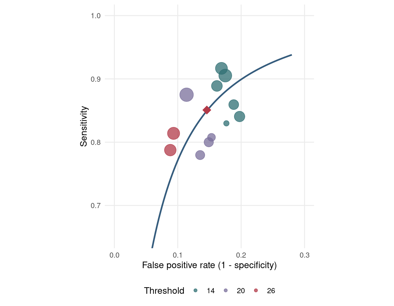
Summary ROC curve (SROC curve) 用來呈現不同 threshold 下 sensitivity 與 specificity 的整體關係。以下用 Moses–Littenberg 型迴歸作為教學示範。正式分析中，HSROC 或 bivariate model 通常更建議。

Code

sroc_data <- troponin_es |>
  mutate(
    s = logit_sens + logit_fpr,
    d = log_dor,
    weight = 1 / se_log_dor^2
  )
moses_fit <- lm(d ~ s, weights = weight, data = sroc_data)
fpr_grid <- seq(0.02, 0.28, length.out = 100)
sroc_curve <- tibble::tibble(fpr = fpr_grid) |>
  mutate(
    logit_fpr = logit(fpr),
    logit_sens = (coef(moses_fit)[1] + (coef(moses_fit)[2] + 1) * logit_fpr) /
      (1 - coef(moses_fit)[2]),
    sensitivity = inv_logit(logit_sens)
  )

ggplot(troponin_es, aes(x = 1 - specificity, y = sensitivity)) +
  geom_point(aes(size = tp + fn, color = factor(threshold)), alpha = 0.75) +
  geom_line(data = sroc_curve, aes(x = fpr, y = sensitivity),
            inherit.aes = FALSE, color = "#355C7D", linewidth = 1) +
  geom_point(data = summary_point, aes(x = fpr, y = sensitivity),
             inherit.aes = FALSE, shape = 18, size = 5, color = "#B23A48") +
  scale_size_continuous(range = c(3, 8), guide = "none") +
  scale_color_manual(values = c("14" = "#2F6F73", "20" = "#7A6F9B", "26" = "#B23A48")) +
  coord_equal(xlim = c(0, 0.30), ylim = c(0.65, 1)) +
  labs(x = "False positive rate (1 - specificity)",
       y = "Sensitivity",
       color = "Threshold") +
  theme_minimal(base_size = 12) +
  theme(legend.position = "bottom", panel.grid.minor = element_blank())

Figure 9.5: 高敏感度 troponin 快速檢測的教學版 summary ROC curve。

Code

dor_forest <- troponin_es |>
  mutate(
    dor_low = exp(log_dor - 1.96 * se_log_dor),
    dor_high = exp(log_dor + 1.96 * se_log_dor),
    study = factor(study, levels = rev(study))
  )

ggplot(dor_forest, aes(x = dor, y = study)) +
  geom_vline(xintercept = 1, linetype = "dashed", color = "grey45") +
  geom_errorbar(aes(xmin = dor_low, xmax = dor_high, color = factor(threshold)),
                orientation = "y", width = 0.18, linewidth = 0.8) +
  geom_point(aes(color = factor(threshold)), size = 3) +
  geom_point(data = tibble::tibble(x = exp(as.numeric(dor_fit$b[1])), y = "Summary DOR"),
             aes(x = x, y = y), inherit.aes = FALSE, shape = 18, size = 4, color = "#B23A48") +
  scale_x_log10() +
  scale_color_manual(values = c("14" = "#2F6F73", "20" = "#7A6F9B", "26" = "#B23A48")) +
  labs(x = "Diagnostic odds ratio (log scale)",
       y = NULL,
       color = "Threshold") +
  theme_minimal(base_size = 12) +
  theme(legend.position = "bottom", panel.grid.minor = element_blank())

Figure 9.6: 各研究的診斷勝算比與隨機效應摘要估計。

9.7 R 工作流程與套件提醒

本章完整 R 腳本儲存在 scripts/chapter9.R。你可以在專案根目錄執行：

Code

/usr/bin/Rscript scripts/chapter9.R

本章可執行內容使用 metafor、mada、ggplot2、dplyr、knitr，目前本機皆已安裝；不需要再安裝額外 R package。mada 適合 frequentist Reitsma/HSROC workflow，meta4diag 則適合 Bayesian bivariate DTA meta-analysis。若在其他電腦重現本章，可使用：

Code

install.packages(c("mada", "meta4diag"))

meta4diag 的模型通常需要較多計算時間與 Bayesian prior 設定；本章把它作為進階延伸，不在主要範例中執行。基本資料整理可如下：

Code

library(meta4diag)
meta4diag_data <- meta4diag::makeData(troponin_mada, model.type = 1)
fit_bayes <- meta4diag::meta4diag(meta4diag_data, seed = 20260630)
summary(fit_bayes)

9.8 小結

診斷準確度統合分析的核心是同時理解 sensitivity 與 specificity。單一 DOR 很方便，但可能隱藏 threshold trade-off。Bivariate model 與 HSROC model 能更自然地處理兩個相關指標與研究間異質性。臨床解讀時，請永遠回到問題本身：這個檢查是用來 rule out，還是 rule in？不同用途需要不同的 sensitivity/specificity 平衡。

9.9 Glossary

中文	English
診斷準確度研究	diagnostic test accuracy study, DTA study
敏感度	sensitivity
特異度	specificity
真陽性	true positive, TP
偽陽性	false positive, FP
偽陰性	false negative, FN
真陰性	true negative, TN
參考標準	reference standard
閾值效應	threshold effect
參考標準偏倚	reference standard bias
驗證偏倚	verification bias
Spectrum effect	spectrum effect
陽性預測值	positive predictive value, PPV
陰性預測值	negative predictive value, NPV
陽性似然比	positive likelihood ratio, LR+
陰性似然比	negative likelihood ratio, LR-
診斷勝算比	diagnostic odds ratio, DOR
連續型 marker	continuous marker
ROC curve	receiver operating characteristic curve
Summary ROC curve	summary ROC curve, SROC curve
Hierarchical model	hierarchical model
Hierarchical summary ROC model	hierarchical summary ROC model, HSROC model
Bivariate model	bivariate model
Reitsma model	Reitsma bivariate model
Bayesian diagnostic test accuracy meta-analysis	Bayesian diagnostic test accuracy meta-analysis
False positive rate	false positive rate
研究間異質性	between-study heterogeneity